
![]()
Uncertainty#
Uncertainty is one of the most important topics in statistics. Visualizing that uncertainty is very critical to expressing these statistical ideas. We’ll explore several ways to display this crutical concept.
Waffle Charts#
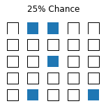
With Random Chance#
import numpy as np


truths = np.random.binomial(1,.25,25)

truths
array([0, 1, 1, 0, 0, 0, 0, 0, 0, 0, 0, 0, 1, 0, 0, 0, 0, 0, 0, 0, 0, 1,
       0, 0, 1])
import matplotlib.pyplot as plt
from matplotlib.patches import Rectangle

fig, axs = plt.subplots(5, 5, constrained_layout=True, figsize=(2, 2))


def hatches_plot(ax,h):
    ax.add_patch(Rectangle((0, 0), 1, 1, fill=h))
    ax.axis('equal')
    ax.axis('off')

for ax, h in zip(axs.flat,truths):
    hatches_plot(ax,h)

fig.suptitle('25% Chance')

plt.show()
With Package#
!pip install pywaffle
Collecting pywaffle
  Downloading pywaffle-0.6.4-py2.py3-none-any.whl (565 kB)
?25l
     |▋                               | 10 kB 21.6 MB/s eta 0:00:01
     |█▏                              | 20 kB 11.3 MB/s eta 0:00:01
     |█▊                              | 30 kB 8.8 MB/s eta 0:00:01
     |██▎                             | 40 kB 7.9 MB/s eta 0:00:01
     |███                             | 51 kB 6.0 MB/s eta 0:00:01
     |███▌                            | 61 kB 7.1 MB/s eta 0:00:01
     |████                            | 71 kB 6.6 MB/s eta 0:00:01
     |████▋                           | 81 kB 6.5 MB/s eta 0:00:01
     |█████▏                          | 92 kB 7.3 MB/s eta 0:00:01
     |█████▉                          | 102 kB 7.0 MB/s eta 0:00:01
     |██████▍                         | 112 kB 7.0 MB/s eta 0:00:01
     |███████                         | 122 kB 7.0 MB/s eta 0:00:01
     |███████▌                        | 133 kB 7.0 MB/s eta 0:00:01
     |████████                        | 143 kB 7.0 MB/s eta 0:00:01
     |████████▊                       | 153 kB 7.0 MB/s eta 0:00:01
     |█████████▎                      | 163 kB 7.0 MB/s eta 0:00:01
     |█████████▉                      | 174 kB 7.0 MB/s eta 0:00:01
     |██████████▍                     | 184 kB 7.0 MB/s eta 0:00:01
     |███████████                     | 194 kB 7.0 MB/s eta 0:00:01
     |███████████▋                    | 204 kB 7.0 MB/s eta 0:00:01
     |████████████▏                   | 215 kB 7.0 MB/s eta 0:00:01
     |████████████▊                   | 225 kB 7.0 MB/s eta 0:00:01
     |█████████████▎                  | 235 kB 7.0 MB/s eta 0:00:01
     |██████████████                  | 245 kB 7.0 MB/s eta 0:00:01
     |██████████████▌                 | 256 kB 7.0 MB/s eta 0:00:01
     |███████████████                 | 266 kB 7.0 MB/s eta 0:00:01
     |███████████████▋                | 276 kB 7.0 MB/s eta 0:00:01
     |████████████████▏               | 286 kB 7.0 MB/s eta 0:00:01
     |████████████████▉               | 296 kB 7.0 MB/s eta 0:00:01
     |█████████████████▍              | 307 kB 7.0 MB/s eta 0:00:01
     |██████████████████              | 317 kB 7.0 MB/s eta 0:00:01
     |██████████████████▌             | 327 kB 7.0 MB/s eta 0:00:01
     |███████████████████             | 337 kB 7.0 MB/s eta 0:00:01
     |███████████████████▊            | 348 kB 7.0 MB/s eta 0:00:01
     |████████████████████▎           | 358 kB 7.0 MB/s eta 0:00:01
     |████████████████████▉           | 368 kB 7.0 MB/s eta 0:00:01
     |█████████████████████▍          | 378 kB 7.0 MB/s eta 0:00:01
     |██████████████████████          | 389 kB 7.0 MB/s eta 0:00:01
     |██████████████████████▋         | 399 kB 7.0 MB/s eta 0:00:01
     |███████████████████████▏        | 409 kB 7.0 MB/s eta 0:00:01
     |███████████████████████▊        | 419 kB 7.0 MB/s eta 0:00:01
     |████████████████████████▎       | 430 kB 7.0 MB/s eta 0:00:01
     |█████████████████████████       | 440 kB 7.0 MB/s eta 0:00:01
     |█████████████████████████▌      | 450 kB 7.0 MB/s eta 0:00:01
     |██████████████████████████      | 460 kB 7.0 MB/s eta 0:00:01
     |██████████████████████████▋     | 471 kB 7.0 MB/s eta 0:00:01
     |███████████████████████████▏    | 481 kB 7.0 MB/s eta 0:00:01
     |███████████████████████████▉    | 491 kB 7.0 MB/s eta 0:00:01
     |████████████████████████████▍   | 501 kB 7.0 MB/s eta 0:00:01
     |█████████████████████████████   | 512 kB 7.0 MB/s eta 0:00:01
     |█████████████████████████████▌  | 522 kB 7.0 MB/s eta 0:00:01
     |██████████████████████████████▏ | 532 kB 7.0 MB/s eta 0:00:01
     |██████████████████████████████▊ | 542 kB 7.0 MB/s eta 0:00:01
     |███████████████████████████████▎| 552 kB 7.0 MB/s eta 0:00:01
     |███████████████████████████████▉| 563 kB 7.0 MB/s eta 0:00:01
     |████████████████████████████████| 565 kB 7.0 MB/s
?25hRequirement already satisfied: matplotlib in /usr/local/lib/python3.7/dist-packages (from pywaffle) (3.2.2)
Requirement already satisfied: kiwisolver>=1.0.1 in /usr/local/lib/python3.7/dist-packages (from matplotlib->pywaffle) (1.4.2)
Requirement already satisfied: pyparsing!=2.0.4,!=2.1.2,!=2.1.6,>=2.0.1 in /usr/local/lib/python3.7/dist-packages (from matplotlib->pywaffle) (3.0.8)
Requirement already satisfied: cycler>=0.10 in /usr/local/lib/python3.7/dist-packages (from matplotlib->pywaffle) (0.11.0)
Requirement already satisfied: python-dateutil>=2.1 in /usr/local/lib/python3.7/dist-packages (from matplotlib->pywaffle) (2.8.2)
Requirement already satisfied: numpy>=1.11 in /usr/local/lib/python3.7/dist-packages (from matplotlib->pywaffle) (1.21.6)
Requirement already satisfied: typing-extensions in /usr/local/lib/python3.7/dist-packages (from kiwisolver>=1.0.1->matplotlib->pywaffle) (4.2.0)
Requirement already satisfied: six>=1.5 in /usr/local/lib/python3.7/dist-packages (from python-dateutil>=2.1->matplotlib->pywaffle) (1.15.0)
Installing collected packages: pywaffle
Successfully installed pywaffle-0.6.4
from pywaffle import Waffle

fig = plt.figure(
    FigureClass=Waffle,
    rows=5,
    columns=10,
    values=[48, 46, 6],
    figsize=(5, 3)
)
plt.show()

pywaffle is actually a pretty cool package for doing this sort of graphic! For my 25% chance above, I’d do something like:
plt.figure(FigureClass = Waffle,
           rows= 5,
           columns = 5,
           values = [5,20],
           colors = ['blue','white'],
           vertical = True,
           facecolor='#DDDDDD' )
plt.show()

The package has lots of options to include some really cool graphics. Here is how many times I biked versus driving this week.
plt.figure(FigureClass=Waffle,
           rows = 5,
           values = [2,3],
           icons = ['bicycle','car'])

plt.show()

Error Bars for Mean#
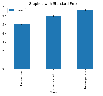
Perhaps the most fundamental concept in error is the mean. We know that the mean will be approximately distributed as normal for a large enough sample size with standard deviation \(\frac s{\sqrt n}\) where \(s\) is the sample standard deviation and \(n\) the sample size. Let’s see that visualized in a bar graph.
import pandas as pa

df = pa.read_csv('https://raw.githubusercontent.com/nurfnick/Data_Viz/main/Data_Sets/iris.csv')

dfgrouped = df.groupby('Class').agg(['mean','std', 'count'])

dfgrouped.SepalLength.plot.bar(y = 'mean',yerr = 'std', legend = False, color = ['purple','red', 'blue'], title = "Error of Standard Deviation")
<matplotlib.axes._subplots.AxesSubplot at 0x7f2a5c169fd0>

import numpy as np
from scipy.stats import t

def SE(std,n):
  return std/np.sqrt(n)


dfgroupedSepalLength = dfgrouped.SepalLength

dfgroupedSepalLength['SE'] = dfgroupedSepalLength.apply(lambda x: SE(x['std'],x['count']), axis = 1)


dfgroupedSepalLength.loc[:,'95%'] = dfgroupedSepalLength.loc[:,'SE']*t.ppf(.975,49)

dfgroupedSepalLength
/usr/local/lib/python3.7/dist-packages/ipykernel_launcher.py:11: SettingWithCopyWarning:
A value is trying to be set on a copy of a slice from a DataFrame.
Try using .loc[row_indexer,col_indexer] = value instead

See the caveats in the documentation: https://pandas.pydata.org/pandas-docs/stable/user_guide/indexing.html#returning-a-view-versus-a-copy
  # This is added back by InteractiveShellApp.init_path()
/usr/local/lib/python3.7/dist-packages/pandas/core/indexing.py:1667: SettingWithCopyWarning:
A value is trying to be set on a copy of a slice from a DataFrame.
Try using .loc[row_indexer,col_indexer] = value instead

See the caveats in the documentation: https://pandas.pydata.org/pandas-docs/stable/user_guide/indexing.html#returning-a-view-versus-a-copy
  self.obj[key] = value
| mean | std | count | SE | 95% | |
|---|---|---|---|---|---|
| Class | |||||
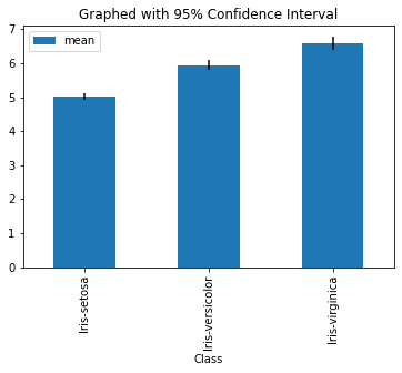
| Iris-setosa | 5.006 | 0.352490 | 50 | 0.049850 | 0.100176 |
| Iris-versicolor | 5.936 | 0.516171 | 50 | 0.072998 | 0.146694 |
| Iris-virginica | 6.588 | 0.635880 | 50 | 0.089927 | 0.180715 |
dfgroupedSepalLength.plot.bar(y = 'mean',yerr = 'SE', title = 'Graphed with Standard Error' )
<matplotlib.axes._subplots.AxesSubplot at 0x7f2a5bb85d10>
dfgroupedSepalLength.plot.bar(y = 'mean',yerr = '95%', title = 'Graphed with 95% Confidence Interval' )
<matplotlib.axes._subplots.AxesSubplot at 0x7f2a5bb0ce90>
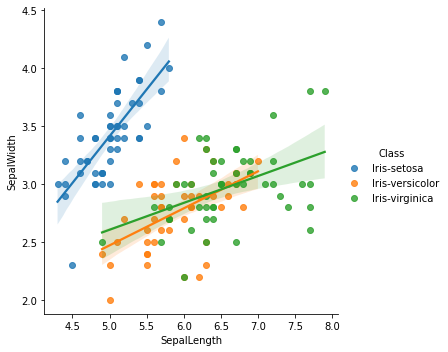
Confidence Interval for Regression#
It is automatically generated with seaborn. It is computed with a bootstrap(!).
import seaborn as sns
import matplotlib.pyplot as plt


sns.lmplot(data = df,
            x = 'SepalLength',
            y = 'SepalWidth',
            hue = 'Class')

plt.show()
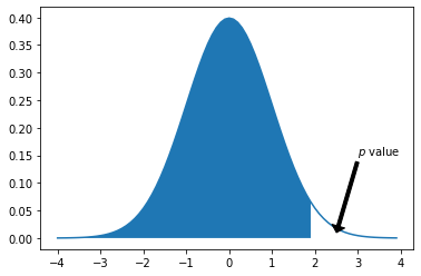
Hypothesis Testing#
from scipy import stats

x = [x for x in np.arange(-4,4,.1)]
x_trunk = [i for i in x if i<2]

plt.plot(x, stats.norm.pdf(x, 0, 1))
plt.fill_between(x_trunk, 0, stats.norm.pdf(x_trunk,0,1))
plt.annotate(r'$p$ value', xy = [2.5,.01],
            xytext = [3,.15],
            arrowprops = dict(facecolor = 'black', width = 3, headwidth = 12, headlength = 6))
plt.show()
Your Turn#
Explain the difference between standard error and confidence intervals.
Use the workout data and graph the average calories by workout type and include the 95% confidence interval.