Regression¶

Introduction¶

Regression is a huge topic but we’ll try to cover the basics here with the idea that you will use regression often in business settings and that all the details will not be needed.

We will mostly focus on the Method of Least Squares here. The idea is to make a prediction and to minimize the error in that prediction by minimizing the sum of the squares of that error:

\[ SSE = \sum_{i=1}^n\left(y_i-\hat {y_i}\right)^2 \]

Derivation¶

To derive the linear regression formula, we assume that $\hat y$ is linear, $$ \hat y = \beta_0 +\beta_1 x $$

Then we plug this into the sum of squares error and take the partial derivatives with respect to $\beta_0$ and $\beta_1$. To minimize we then set those derivatives to zero and solve the system.

\[ \nabla SSE(\beta_0,\beta_1) = \left( \sum -2(y_i-\beta_0 - \beta_1 x_i) , \sum -2(y_i-\beta_0 - \beta_1 x_i)x_i \right) \]

Setting each of these to zero and simplifying the summations, we arrive at $$ \sum y_i = n\beta_0 +\beta_1\sum x_i $$ \sum x_iy_i = \beta_0\sum x_i +\beta_1\sum x^2_i $$

Eliminating and solving, we see that $$ \beta_1 = \frac{n\sum x_iy_i - \sum x_i \sum y_i}{n\sum x_i^2 - (\sum x_i)^2} $$

and $$ \beta_0 = \frac{\sum y_i - \beta_1\sum x_i}n $$

Some times these are written using the bar notation, $\bar x = \frac{\sum x_i}n$

\[ \beta_0 = \bar y - \beta_1\bar x \]

\[ \beta_1 = \frac{\bar{xy}-\bar x\bar y}{\bar{x^2} - \left(\bar x\right)^2} \]

Example¶

Given the points $(0,4),(3,6),(7,8),(2,5)$, find the linear regression.

x = [0,3,7,2]
y = [4,6,8,5]
n = len(x)

meanx = sum(x)/n
meany = sum(y)/n
sumsquarex = 0
for i in range(n):
  sumsquarex += x[i]**2
sumsquarex /= n

xy = 0
for i in range(n):
  xy +=x[i]*y[i]
xy/=n

b1 = (xy - meanx*meany)/(sumsquarex-meanx**2)
b1

0.5769230769230769

b0 = meany - b1*meanx
b0

4.019230769230769

def line(x):
  return b1*x+b0

import numpy as np
import matplotlib.pyplot as plt

xs = np.linspace(0,8,100)
ys = line(xs)

plt.plot(xs,ys)
plt.scatter(x,y)

<matplotlib.collections.PathCollection at 0x7c7345e77c70>

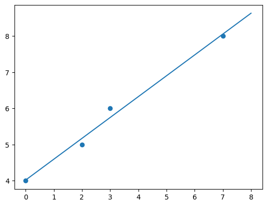
Fits the line very well! You should be asking yourself why I didn’t use a built-in for this. Well I should. I picked scipy for my package as the code is easier to explain than scikit-learn.

from scipy import stats

stats.linregress(x,y)

LinregressResult(slope=0.5769230769230769, intercept=4.019230769230769, rvalue=0.9944903161976938, pvalue=0.005509683802306207, stderr=0.04300130725961148, intercept_stderr=0.16929631597749104)

We see that the slope $\beta_1$ and intercept $\beta_0$ agree with our above calculation.

$r$ Value¶

The $r$ value is an evaluation of the strength of the fit. $r$ is called the correlation coefficient and is calculated as $$ r_{xy} = \frac{n\left(\bar{xy}-\bar x\bar y\right)}{(n-1)s_xs_y} $$

Where $s_x$ is the sample standard deviation $s_x = \sqrt{\frac1{n-1}\sum (x_i-\bar x)^2}$

Let’s repeat our example and compute this. The only new thing required is the sample standard deviations.

sx = 0

for i in x:
  sx+= (i-meanx)**2

sx/=len(x)-1
sx = (sx)**(1/2)


sy = 0

for i in y:
  sy+= (i-meany)**2

sy/=len(y)-1
sy = (sy)**(1/2)

r = len(x)*(xy - meanx*meany)/((len(x)-1)*sx*sy)

r

0.9944903161976939

Perhaps a better way to consider the correlation coefficient in the terms of the linear fit is to see it under the regression. The correlation coffiecient can be shown to be

\[ r^2 = \frac{SSR}{SST} = \frac{\sum(\hat y_i-\bar y)^2}{\sum(y_i-\bar y)^2} \]

So it is giving us a measure of how much the regression varies from the mean compared to the data varying from the mean. Let’s compute this with our data just to see that these are equivalent.

SSR = 0
SST = 0

for i in x:
  SSR += (line(i)-meany)**2
for i in y:
  SST += (i-meany)**2

r = (SSR/SST)**(1/2)
r

array([1.28388148, 1.28388148, 1.28388148])

Multiple Regression¶

For multiple regression, we will ask that there is some linear transformation from $\vec x$ to $y$. So we want $$ y = \beta_1x_1 +\beta_2x_2 +\cdots +\beta_n x_n $$

We can accomplish this by considering all the $y$ in a column matrix and all the $x$ in a matrix then $$ Y = X\mathbf{\beta} $$

But we want to find the $\mathbf{\beta}$ that solve this equation. We assume that $X$ is rank $n$, then $X^TX$ is invertible so $$ X^TY = X^TX\beta $$ so $$ \beta = \left(X^TX\right)^{-1}X^TY $$

Example¶

Let’s use the same example from above and compute the linear regression in a multiple regression system. To do this, you add the intercept by creating a column of 1’s in the $X$ matrix, np.ones is perfect for this. Matrix multiplication is in the numpy package with @ and matrix inverse can be done with np.linalg.inv

x = np.array([[0,3,7,2],np.ones(4)]).T
y = np.array([4,6,8,5])

print(x)

[[0. 1.]
 [3. 1.]
 [7. 1.]
 [2. 1.]]

a,b = np.linalg.inv(x.T@x)@(x.T@y)
print(a,b)

0.5769230769230764 4.019230769230767

Example with Categorical Variables¶

I am going to add a categorical variable to my baby example and show how we would include that. $(0,4,yes),(3,6,no),(7,8,yes),(2,5,no)$,

Since my dataset is tiny, I could do it by hand but what fun would that be?

x = np.array([[0,3,7,2],['yes','no','yes','no']]).T
y = np.array([4,6,7,5])

x

array([['0', 'yes'],
       ['3', 'no'],
       ['7', 'yes'],
       ['2', 'no']], dtype='<U21')

I have printed the column of categorical variables. I will next change it via a one-hot-encoding. Again I could use the scikit-learn package but I am not.

I grab the column that has the categorical variables, find the different values it can be and then add columns to the x matrix with the indicator variable.

allTheOptionsForCategrocial = np.unique(x[:,1])
allTheOptionsForCategrocial

array(['no', 'yes'], dtype='<U21')

for i in allTheOptionsForCategrocial:
  x = np.append(x,1*(x[:,1] == i)[...,None], 1)

array([['0', 'yes', '0', '1'],
       ['3', 'no', '1', '0'],
       ['7', 'yes', '0', '1'],
       ['2', 'no', '1', '0']], dtype='<U21')

I’ve added the columns for the indicator. Now I will remove the categorical one so all entries are numeric.

x = x[:,[0,2,3]]

x

array([['0', '0', '1'],
       ['3', '1', '0'],
       ['7', '0', '1'],
       ['2', '1', '0']], dtype='<U21')

Some reason everything is a char so I’ll convert back to floats.

x = np.float64(x)
x

array([[0., 0., 1.],
       [3., 1., 0.],
       [7., 0., 1.],
       [2., 1., 0.]])

Time for the formula!

result = np.linalg.inv(x.T@x)@(x.T@y)

result

array([0.44, 4.4 , 3.96])

Interpreting this insists that slope for numeric is 0.44 but if you have a ‘no’ you have intercept of 4.4 where as if you have a ‘yes’ your intercept is 3.96. This answer is very similar to before!

We compute the multiple coeffiecint of determination, $R^2$ value as $\frac{SSR}{SST}$

def predict(x):
  return sum(x[i]*result[i] for i in range(3))

SSR = 0
SST = 0
meany = sum(y)/n

for i in x:
  SSR += (predict(i)-meany)**2
for i in y:
  SST += (i-meany)**2

r = (SSR/SST)**(1/2)
r

0.9838699100999083

Other Regressions¶

Exponential¶

Many other regressions can be expressed as the linear regression. For example, you suspect an exponential growth.
$$ y = ce^{ax} $$ It is enough to take the log of your output $y$ and fit a linear regression since $$ \log y = \log(ce^{ax}) = \log c + ax = \beta_0+\beta_1x. $$

So transform your $y$ values via the logarithm. Fit with a linear regression. Make sure to interpret your predictions correctly when making them.

Polynomial¶

Sometime we might be interested in a polynomial expansion, $\hat y = \beta_0+\beta_1x+\beta_2 x^2+\cdots+\beta_nx^n$. To deal with this, we transform our x variable, computing $x^2$, $x^3$, etc. Add these new columns to the multiple regression matrix and compute the multiple linear regression. Again we should be careful of predcitions and confidence intervals as they are not the same as in the linear case.

Logistic Regression¶

Often we are interested in assigning a probability of a certain outcome based on another variable. Consider the example of passing your operations research test based on how many hours you studied. Below is survey results of number of hours studied and an indeicator for passing $$ (10,1),(5,1),(5,0),(1,0) $$

We want to be able to figure out your likelyhood of passing based on the number of hours you study.

x = np.array([[10],[5],[5],[1]])
y = np.array([1,1,0,0])

This was especially difficult in that it requires an advanced numerical method, not simply a transformation like the above. Therefore I will use the scikit-learn package.

from sklearn.linear_model import LogisticRegression

logreg = LogisticRegression()
logreg.fit(x, y)

LogisticRegression()

In a Jupyter environment, please rerun this cell to show the HTML representation or trust the notebook.
On GitHub, the HTML representation is unable to render, please try loading this page with nbviewer.org.

xs = np.linspace(0,10,100)
xs = xs.reshape(100,1)
ys = logreg.predict_proba(xs)

plt.plot(xs,ys)
plt.scatter(x,y)

<matplotlib.collections.PathCollection at 0x7c733d54c1c0>

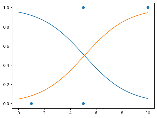
There is clearly some weirdness here. Partially this is the lack of data. But you should get the idea on how to fit. The reshaping of the np.arrays was annoying but nesseccary to get the fit done.

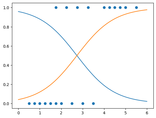
I want to repeat the regression with some data I got from wikipedia.

x = [ 	0.50, 	0.75, 	1.00, 	1.25, 	1.50, 	1.75, 	1.75, 	2.00, 	2.25, 	2.50, 	2.75, 	3.00, 	3.25, 	3.50, 	4.00, 	4.25, 	4.50, 	4.75, 	5.00, 	5.50]
y = [	0 ,	0 ,	0 ,	0 ,	0 ,	0 ,	1 ,	0 ,	1 ,	0 ,	1 ,	0 ,	1 ,	0 ,	1 ,	1 ,	1 ,	1, 	1, 	1 ]

x = np.array(x).reshape(20,1)

logreg = LogisticRegression()
logreg.fit(x, y)

xs = np.linspace(0,6,100)
xs = xs.reshape(100,1)
ys = logreg.predict_proba(xs)

plt.plot(xs,ys)
plt.scatter(x,y)

<matplotlib.collections.PathCollection at 0x7c733d5c1d20>

Operations Research OER

Regression¶

Introduction¶

Derivation¶

Example¶

\(r\) Value¶

Multiple Regression¶

Example¶

Example with Categorical Variables¶

Other Regressions¶

Exponential¶

Polynomial¶

Logistic Regression¶