Dynamic Programming¶

Introduction¶

In the last three decades, industries have shifted to a more tech friendly environment. This created a higher demand for programmers, scalable applications, and the ability to improve the applications that consumers and employees use daily. This created a demand for finding better ways to optimize programmable applications and increase performance and productivity. Humans are problem solvers, always trying to devise the best way to find a solution. People complete their task in different ways. Some solutions are effective but take time. While other solutions may be finished quickly, the job is sloppy. The same thing can be said about programming code. The goal is to find both an optimal and time efficient solution that can limit the run time of the application and give the user more time to complete other tasks. An excellent method to complete this goal is dynamic programming.

Dynamic programming is a method created by Richard Bellman in the 1950s. The top tech companies, such as Google, Wal-Mart, and Amazon, all use the dynamic programming method. They even use interview questions to test the knowledge, critical thinking, and analytical skills of their candidates to see how much they understand and comprehend about dynamic programming. This chapter will break down and give a generalization of what dynamic programming is, how it is applied to code, and will break dynamic programming down into three parts: recursion, memoization, and the difference between bottom-up and top-down approach.

Dynamic Programming is mainly an optimization over plain recursion. Recursion is when a program calls back on the same function or variable that has been declared.

#Note how the function calls on itself and we have another call to return recursion(). This is one of the most basic examples of recursion.
def recursion(): 
    print("You could not live with your own failure. Where did that bring you? Back to me. --Thanos")
    return recursion()
    
#recursion() 
#Removing the comment from above will cause the recursion function to loop infinitely because it will keep calling on itself.

Recursion

Figure 1: Visual example of recursion

Recursion: Fibonacci Sequence¶

Example 1: Let’s take a look at a real example of recursion.

Let’s try to understand this by taking an example of Fibonacci numbers.

Fibonacci (n) = 1; if n = 0 Fibonacci (n) = 1; if n = 1 Fibonacci (n) = Fibonacci(n-1) + Fibonacci(n-2)

The first few numbers in this series will be: 1, 1, 2, 3, 5, 8, 13, 21… and so on!

A code for the Fibonacci Sequence is using pure recursion:

def fib(n):
    if n==1 or n==2:
        return 1
    else:
        fibSeq = fib(n-1) + fib(n-2)
    return fibSeq

print(fib(1))

print(fib(20))

Time complexity is defined by the amount of time it takes for the program to run.

Space complexity is defined as how much space an algorithm or program takes up.

T(n) = T(n-1) + T(n-2) is exponential. We can observe that this implementation does a lot of repeated work (see the following recursion tree). This is a bad implementation for nth Fibonacci number. Since the Fibonacci method does only a constant amount of work, the time complexity is proportional to the number of calls to Fibonacci Sequence, that is the number of nodes in the recursive call tree.

The recursive call tree is a binary tree, and for fib(n) it has n levels. Therefore, the maximum number of nodes in this tree is 2n−1. The time complexity is thus \(O(2^n)\).

The Fibonacci Sequence requires just a constant amount of memory, but each recursive call adds a frame to the system’s call stack. Thus, the algorithm uses space proportional to the maximum number of the Fibonacci Sequence frames that can be simultaneously on the call stack. This equals the number of levels of the recursive call tree.

For fib(n), the number of levels of the recursive call tree is n. Thus, the space complexity of the algorithm is \(O(n)\).

Wherever there is a recursive solution that has repeated calls for certain types of input, we can optimize it using dynamic programming. The idea is to simply store that results of subproblems, so that we do not have to re-compute them when needed later. This simple optimization reduces time complexities from exponential to polynomial. Since dynamic programming is optimizing problems by breaking down the algorithm into subproblems, it helps prevent each subproblem from being solved more than once which can be achieved by running a recursive function once and storing in memory this is called memoization.

Memoization: Matrix Chain¶

Memoization prevents continuous solving of the same recursive subproblems by creating a ‘sticky note’ like save-state per inputs to be called for later calculations. This programming technique takes advantage of the CPU’s cache and stores those more time-consuming calculations to later be used when called on throughout the solutions.

Memoization

Figure 2: Memoization: Recursive calls are stored in an array. With sticky notes, information gets written down and the sticky notes get be placed next to each other. This is the same way an array stores its data in memory.

Memoization should only be used for recursive calculations so that when requesting an output it will stay consistent each time calculations are executed. If not, the program would lose its efficiency and gained advantages as memoization would in the end take up more CPU cycle times to verify its cache stored data in verifying whether the output would be the same or not. Global variables would also greatly influence or break a memoized function. A different algorithm would be much more acceptable.

Example 2: Memoization

Objective: To efficiently calculate a sequence of matrices

Sidenote: Not focusing on the multiplication itself but finding the best route to make the calculations. In some problems, where you put parentheses can either minimize or maximize the number of operations needed to find a solution.

The problem in question:

ABCD = A(BCD) = (AB)(CD) = (AD)(BC) = ALL PRODUCE SAME OUTPUT

A = 10 x 20 B = 20 x 30 C = 30 x 40 D = 40 x 60

Here we would like to demonstrate difference in the number of operations needed when you change up the sequence in which you attempt to calculate the matrices.

(AB)C -> (10 x 20 x 30) + (10 x 30 x 40) = 6000 + 12,000 = 18,000 operations {10, 20, 30, 40}

A(BC) -> (20 x 30 x 40) + (10 x 20 x 40) = 24,000 + 8,000 = 32,000 operations {10, 40, 40, 40}

Calculating (AB)C would take almost half the time of calculating A(BC)

#To show operations needed for certain sequence of matrices
import sys
  
def MtxChainOrder(p, n):
    m = [[0 for x in range(n)] for x in range(n)]
  
    for i in range(1, n):
        m[i][i] = 0
  
    for Lst in range(2, n):
        for i in range(1, n-Lst + 1):
            j = i + Lst-1
            m[i][j] = sys.maxsize
            for k in range(i, j):
  
                q = m[i][k] + m[k + 1][j] + p[i-1]*p[k]*p[j]
                if q < m[i][j]:
                    m[i][j] = q
  
    return m[1][n-1]

ele = int(input("Enter how many elements : "))
lst = list(map(int,input("\nEnter Matrices: ").strip().split()))[:ele]
size = len(lst)


print("\nMinimum number of operations for Matrices entered is " +
       str(MtxChainOrder(lst, size)))

#To represent ideal sequence for most efficient calculation 
array = [10, 20, 30, 40]
size2 = len(array)

print("\nMinimum number of operations possible: ", MtxChainOrder(array, size2))

#How to input: 
#Enter how many elements :  
#Enter 4

#Enter Matrices:  
#Enter 10 20 30 40

#Try it with other examples.

Enter how many elements :  4

Enter Matrices:  10 20 30 40

Minimum number of operations for Matrices entered is 18000

Minimum number of operations possible:  18000

Time complexity is \(O(n^3)\).

Top-down Recursion & Bottom-Up: The Rod Cutting Problem¶

Recursion and memoization both take a top-down approach to solving the problem. This means that the problem is looked at as a whole and is broken down into pieces, examining each piece to see how it makes a whole. Top-down can even go further by breaking down the parts into sub subparts. The main languages that also focus on top-down approach are COBOL, Fortran, and C.

Take a look at a plastic model car for example. For top-down we will start by looking at the model car(the root). Because top-down is a decomposition process, we will break the model car down into pieces. You will have many parts: the engine, wheels, the body, and the interior. All these items are separate, but they end up forming the model car. Because they are separate, this can cause redundancy and communication errors within the program.

In most cases, it is better to take a bottom-up approach rather than a top-down approach. Bottom-up has a different approach, it uses composition. Instead of starting from the root, it starts from the bottom, the smallest variable types, and moves upward towards the root. This means that we will build it from the ground up. In the model car example, this would be like pulling the model out of the box. All the pieces are connected, but it still needs to be assembled. The pieces represent the subproblems and the sub subproblems. In objected-oriented programming we can define the model car as a class, meaning that all pieces are no longer separated but in constant communication and reduce redundancy. Good examples for bottom-up are object-oriented languages; languages like C++, C#, and Java, all use the bottom-up approach because the object is always identified first. Finally, once we add each piece and put all the pieces together, we will have a functional model car.

Parse Tree

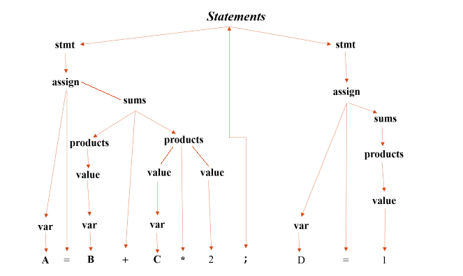
Figure 3: Parse tree with the root called “Statements”.

Top-Down Parse Tree

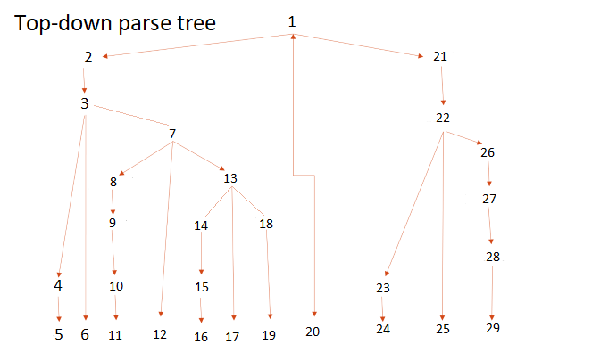
Figure 4: Top-down parse tree. Look at the numerical value and notice how it descends breaking the parse tree down, piece by piece.

Bottom-up Parse Tree

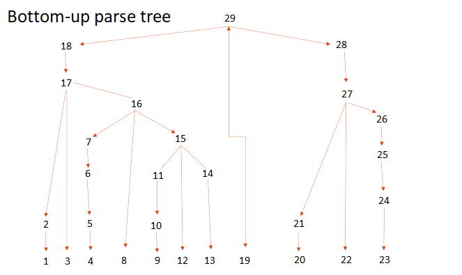
Figure 5: Notice how the bottom-up parse tree tries to compile all pieces from the bottom before it makes its way to the next tier. It is always building every piece to the root.

Example 3: Recursion and Bottom-up.

The Rod Cutting Problem is basic. There is n length of a rod. The seller is wanting to maximize profit. For each length of n there can be a price of i that can represent each length. The seller wants to know what the optimal price is. Should they cut the rod into pieces or sell the rod as it is.

Rod Cut Ex

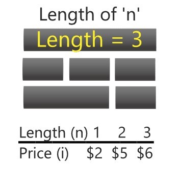
Figure 6: Rod Cutting Example

Example: Let’s say the seller has a rod with the length of 3. The price for length 1 is 2 dollars, length 2 is 5 dollars, and length 3 is 6 dollars.

If the seller wanted to cut the rod into 3 lengths of 1 then each rod would equal 2 dollars each making the profit 6 dollars. This would be equal to the price of the rod if it was not cut at all. If the seller were to cut the rod at a length of 1 and a length of 2, the seller can sell the rod at the price of 7 dollars instead of 6 dollars.

The rod at the length of 3 is very easy to compute, but as the bigger the rod gets in length the more complicated it becomes to solve. Therefore, it is imperative that in a dynamic program problem like the Rod Cutting Problem is optimized because if not it can drastically slow down the time complexity.

Below is an example of a recursive function.

import time
start_time = time.time()

import sys #This is used to call max = -inf

#Recursive function
def RodCutting(length, price):
    
    if length == 0:
        return 0

    maxValue = -sys.maxsize

    for i in range(1, length + 1):

        cost = price[i - 1] + RodCutting(length - i, price)

        if cost > maxValue:
            maxValue = cost

    return maxValue

Time complexity is \(O(n^n)\)

start_time = time.time() #This calls for a new function of time that will only check this code.

print('Maximum profit for rod is: ', RodCutting(3, [2, 5, 6]))

print("--- %s seconds ---" % (time.time() - start_time)) #Will print out the time in a tenth of a second.

Maximum profit for rod is:  7
--- 0.0 seconds ---

start_time = time.time() #This calls for a new function of time that will only check this code.

print('Maximum profit for rod is: ', RodCutting(10, [2, 4, 5, 6, 7, 8, 9, 10, 12, 15]))
 
print("--- %s seconds ---" % (time.time() - start_time)) #Will print out the time in a tenth of a second.

Maximum profit for rod is:  20
--- 0.0005002021789550781 seconds ---

Rod Cut L=3

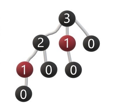
Figure 7: Recursion tree. Length = 3.

Above is a recursion tree with the length of 3. Each number represents a subproblem and it clearly shows that the recursion function is overlapping the subproblems.

Below is another example of a recursion tree. Again, the subproblems are overlapping, but the number of times it needs to run a subproblem is increasing by \(n^2\).

Rod Cut L=4

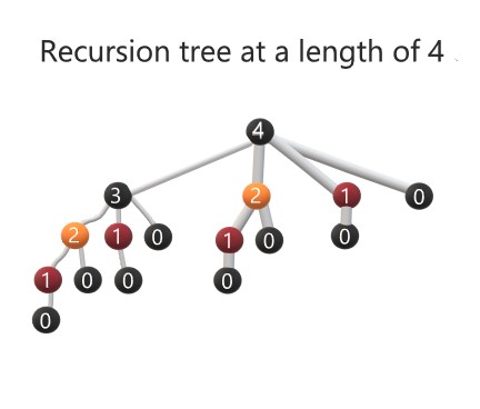
Figure 8: Recursion Tree with a length = 4.

Below is the bottom-up approach. Like memoization this uses an array to store our recursive and adds for loops to quickly run the function.

#Bottom-Up function
def BotUpRodCutting(length, price):
    
    arr = [0] * (length + 1)
    
    for i in range(1, length + 1):
        for j in range(1, i + 1):
            arr[i] = max(arr[i], price[j - 1] + arr[i - j])
            
    return arr[length]
 
    return maxValue

start_time = time.time() #This calls for a new function of time that will only check this code.

print('Maximum profit for rod is ', BotUpRodCutting(3, [2, 5, 6]))

print("--- %s seconds ---" % (time.time() - start_time)) #Will print out the time in a tenth of a second.

Maximum profit for rod is  7
--- 0.0 seconds ---

Time complexity is \(O(n^2)\)

BU Rod Cut L=4

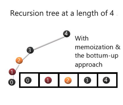
Figure 9: Bottom-Up Tree with a length = 4.

Finally, based on the image above, the run time is reduced significantly because now the recursive subproblems are only being ran once, and are now being stored into memory. Now, the program can go back and review the subproblem that are now stored in an array.

Dynamic programming is a method to increase functionality by optimizing and improving time complexity in code that makes recursive calls. Because the values are not being stored, the recursive calls are constantly being repeated. This performance can slow down run time in a program based on the number of calculations that are being repeated. Using memoization, allows a program to store recursive calls into arrays and store the data. The recursive calls are now stored in memory which eliminates multiple functions calls of the same value. Memoization is effective in increasing time complexity and performance, but it still makes recursive calls and depending on the program can create an error based on the number of calls. To correct issues of recursing, performance can be further increased by changing the approach from top-down to a bottom-up approach. Bottom-up looks at subproblems and composes the program from the bottom to the root. This reduces redundancies and provides clearer communication for the program. Ultimately, increasing performance and functionality, allowing applications to call bigger or larger values quickly and effectively.

How it All Fits Together¶

Fibonacci Sequence¶

Example 4: In this example there are three different Fibonacci Sequences coded: recursive, memoized, and bottom-up. The importance of this code is to see and understand how it works.

First, is the recursive function. This code will call on itself multiple times. This creates redundancy because the sequence will continue to run old numbers of n because there is not any recursive call that is being stored.

#Recursive function
def fib(n):
    if n==1 or n==2:
        return 1
    else:
        fibSeq = fib(n-1) + fib(n-2)
    return fibSeq
        

Run the code above and test the next 3 inputs.

start_time = time.time() #This calls for a new function of time that will only check this code.

print(fib(1)) #Fibonacci Sequence 

print("--- %s seconds ---" % (time.time() - start_time)) #Will print out the time in a tenth of a second.

1
--- 0.0 seconds ---

start_time = time.time() #This calls for a new function of time that will only check this code.

print(fib(20)) #Fibonacci Sequence 

print("--- %s seconds ---" % (time.time() - start_time)) #Will print out the time in a tenth of a second.

6765
--- 0.002000570297241211 seconds ---

start_time = time.time() #This calls for a new function of time that will only check this code.

print(fib(35)) #Fibonacci Sequence 

print("--- %s seconds ---" % (time.time() - start_time)) #Will print out the time in a tenth of a second.

9227465
--- 2.0653629302978516 seconds ---

Notice how fib(35) starts to take a lot longer to display the value of the 35th number in the Fibonacci Sequence.

How can this be fixed? It is important that in the code, the redundancy is reduced. This is where memoization comes into play. Memoization allows the recursive calls to be stored in an array. This eliminates repeat calls for the same n value.

#Memoization function
def mFib(n, mArray):
    if mArray[n] is not None:
        return mArray[n]
    if n==1 or n==2:
        return 1
    else:
        fibSeq = mFib(n-1, mArray) + mFib(n-2, mArray)
    mArray[n] = fibSeq
    return fibSeq

def fibMArray(n):
    mArray = [None] * (n + 1)
    return mFib(n,mArray)

Run the code above and test the next 3 inputs.

start_time = time.time() #This calls for a new function of time that will only check this code.

print(fibMArray(35)) #Fibonacci Sequence 

print("--- %s seconds ---" % (time.time() - start_time)) #Will print out the time in a tenth of a second.

9227465
--- 0.0 seconds ---

start_time = time.time() #This calls for a new function of time that will only check this code.

print(fibMArray(400)) #Fibonacci Sequence 

print("--- %s seconds ---" % (time.time() - start_time)) #Will print out the time in a tenth of a second.

176023680645013966468226945392411250770384383304492191886725992896575345044216019675
--- 0.0004999637603759766 seconds ---

#This is commented out because it will cause a recursion error. To run this example remove the '#' in fron of fibMArray(4000).
#Time was not added to this line of code because it will error out.

#fibMArray(4000) 

This is meant to create an error, even though we are using memoization, there are still too many recursive functions being called which caused this code to error out.

To fix this problem and eliminate more redundancy, the Fibonacci Sequence can be further improved by using the bottom-up approach. Not only is the code much simpler for this program, but now the run time and functionality of the program has been increased significantly.

Note: The main difference between memoization and the bottom-up approach is that memoization still uses recursive calls to the n-1 and n-2 portion of the Fibonacci Sequence. Bottom-up stores the n-1 and n-2 into an array which eliminates the amount of recursive calls that need to be made by the computer.

#Bottom-up function
def B_UFib(n):
    if n==1 or n==2:
        return 1
    B_UArray = [None] * (n+1)
    B_UArray[1] = 1
    B_UArray[2] = 1
    for i in range(3, n+1):
        B_UArray[i] = B_UArray[i-1] + B_UArray[i-2]
    return B_UArray[n]

Run the code above and test the next three inputs.

start_time = time.time() #This calls for a new function of time that will only check this code.

print(B_UFib(1)) #Fibonacci Sequence 

print("--- %s seconds ---" % (time.time() - start_time)) #Will print out the time in a tenth of a second.

1
--- 0.0 seconds ---

start_time = time.time() #This calls for a new function of time that will only check this code.

print(B_UFib(35)) #Fibonacci Sequence 

print("--- %s seconds ---" % (time.time() - start_time)) #Will print out the time in a tenth of a second.

9227465
--- 0.0 seconds ---

start_time = time.time() #This calls for a new function of time that will only check this code.

print(B_UFib(4000)) #Fibonacci Sequence 

print("--- %s seconds ---" % (time.time() - start_time)) #Will print out the time in a tenth of a second.

39909473435004422792081248094960912600792570982820257852628876326523051818641373433549136769424132442293969306537520118273879628025443235370362250955435654171592897966790864814458223141914272590897468472180370639695334449662650312874735560926298246249404168309064214351044459077749425236777660809226095151852052781352975449482565838369809183771787439660825140502824343131911711296392457138867486593923544177893735428602238212249156564631452507658603400012003685322984838488962351492632577755354452904049241294565662519417235020049873873878602731379207893212335423484873469083054556329894167262818692599815209582517277965059068235543139459375028276851221435815957374273143824422909416395375178739268544368126894240979135322176080374780998010657710775625856041594078495411724236560242597759185543824798332467919613598667003025993715274875
--- 0.0014998912811279297 seconds ---

As we can see the time and space complexity is further optimized by using bottom-up than if we used recursion or memoization.

Conclusion¶

Dynamic Programming is incredibly important. Not only does it help change the way people can think to solve a problem, but it helps further optimize programs to be more efficient and handle data more quickly. Using recursion and having the computer calculate a recursive function can bog down the computers space complexity, drastically affecting its time complexity too. Using memoization is a useful tool to help store the recursive data and limit the number of times that the recursive calls must run. However, not all recursive calls completely stop when using memoization and the actual code for using memoization can be tricky. To further improve the code, we can take a different approach and look at building it from the ground up instead of breaking it apart. This is when bottom-up comes into play. We can use more loops and an additional array function to call and store more recursive functions that would have been missed by memoization. In some cases, memoization and bottom-up share the same time complexity, but overall, bottom-up proves to be the most effective when looking at subproblems and trying to find an optimal path.

Operations Research OER

References

Cormen, Thomas H., et al. Introduction to Algorithms. 3rd ed., Massachusetts Institute of Technology, 2009, pp. 30-413.
Uploaded by CS Dojo. “What Is Dynamic Programming and How to Use It.” YouTube.com, YouTube(Owned by Google), 13 Dec. 2017, www.youtube.com/watch?v=vYquumk4nWw. The channel owner of “CS Dojo” has not fully released his name most likely for privacy reasons.
“Cutting a Rod: DP-13.” GeeksforGeeks, GeeksforGeeks, 8 Oct. 2021, https://www.geeksforgeeks.org/cutting-a-rod-dp-13/.
“Difference between Bottom-up Model and Top-down Model.” GeeksforGeeks, GeeksforGeeks, 22 Oct. 2020, https://www.geeksforgeeks.org/difference-between-bottom-up-model-and-top-down-model/.
Dreyfus, Stuart. “RICHARD BELLMAN ON THE BIRTH OF DYNAMIC PROGRAMMING.” Operations Research, vol. 50, no. 1, INFORMS, 2002, pp. 48–51.
“Dynamic Programming - GeeksforGeeks.” GeeksforGeeks, www.geeksforgeeks.org/dynamic-programming/. Accessed 16 Sept. 2021.
“Rod Cutting Problem.” Techie Delight, 29 Sept. 2021, https://www.techiedelight.com/rod-cutting/. Accessed 10 Oct. 2021.
“Program for Fibonacci Numbers.” GeeksforGeeks, 31 Aug. 2021, www.geeksforgeeks.org/program-for-nth-fibonacci-number/.
Weibel, Daniel. “Recursion and Dynamic Programming.” Recursion and Dynamic Programming, 9 Nov. 2017, weibeld.net/algorithms/recursion.html.
Problems
Beginner level:
In your own words, explain what recursion is. Provide a small example.
What does memoization store? How is it stored?
Going back to the model car analogy, create your own analogy that explains the process of top-down and bottom up approach.
Intermediate level:
Following the Rod Cutting Examples, write additional code using the bottom-up function that also displays the cut lengths of the maximum rod.
In the Fibonacci Sequence example, is the bottom-up function the most optimal example? Explain why or why not.
Why is it important to improve time and space complexity?
When working on a project, how can dynamic programming benefit the project?
Advance level:
Given a gold mine of n*m dimensions. Each field in this mine contains a positive integer which is the amount of gold in tons. Initially the miner is at first column but can be at any row. The miner can move only (right->,right up /,right down) that is from a given cell, the miner can move to the cell diagonally up towards the right or right or diagonally down towards the right. Find out maximum amount of gold the miner can collect.
Given two strings; str1, str2, and the below operations, can be performed on str1. Find minimum number of edits (operations) required to convert ‘str1’ into ‘str2’.
Insert
Remove
Replace All of the above operations are of equal cost.
In python, write the memoized version of the rod cutting problem.
Pseudo code example:
MemoizedRodCutting(n,p)
1. Let r[0... n] be a new array
2. for i = 0 to n
3.     r[i] = -infinity
4. return MemoizedCutRod(n,p,r)
MemoizedCutRodFun(n,p,r)
1. if r[n] >= 0
2.    return r[n]
3. if n == 0
4.      q == 0
5. else q = -infinity
6.      for i = 1 to n
7.          q = max(q, p[i] + MemoizedCutRodFun(n - i,p,r))
8. r[n] = q
9. return q
Authors
Principal authors of this chapter were: B.Roy, D.L.Castaneda, & T.A.Wood
Contributors: N.C.Jacob