![]()
Transportation Theory
Introduction
The main motivation is to optimize the transportation of products. Transportation is something that is used all over the world all the time. Transport is used by every society and business. In fact, people are still trying to figure out the optimal way to transport. This is amazing considering how transport has been around for a long time. The theoretical foundation was laid by French mathematician Gaspard Monge in 1781! With how important transportation is and how it is continuing to evolve, we believe that is important for everyone to have a solid grasp on this idea
History
Monge-Kantorovich optimal transport, or Monge-Kantorovich optimization, has a rich history. As we stated in the introduction, it dates back to the classic 1781 paper of Monge, “Memoire sur la theorie des deblais et des remblais”, related to the most economical way of moving soil from one area to the other. In its most concrete form its application for military and economic purposes is obvious. Monge specified the theory in terms of minimizing the L1 norm of the distance transported. The L2 theory came later, leading to the Monge-Ampere equation, an important nonlinear partial differential equation. The theory received a boost in the 1940’s when Kantorovich generalized it to what is now known as the Kantorovich dual problem, and showed how to deal with it using his newly developed method of linear programming.
Theory
The main idea of the optimal transportation problem is that we are trying to minimize cost of transporting products while satisfying the supply and demand restrictions. We set up the problem with m sources and n destinations, called nodes. These nodes are connected by arcs. These arcs represent the transportation cost between each node. Transportation is composed of suppliers of transport services and users of these services. Well-functioning transport markets should allow the transport supply to meet transport demand to satisfy transport needs for mobility. Mobility could not occur or would not occur in a cost-efficient manner. This interdependency can be considered according to two concepts, which are transport supply and demand. Supply is expressed in terms of infrastructures (capacity), services (frequency), and networks (coverage). Capacity is often assessed in static and dynamic terms where static capacity represents the amount of space available for transport. Transport demand similar to transport supply, it is expressed in terms of the number of people, volume, or tons per unit of time and distance.
Examples
Example 1
Let us look at it in the simplest way possible. We have one factory and two warehouses. We have a supply of 16 at the factory. There is also a demand of 11 at warehouse one and a demand of 5. It costs 7 dollars a unit to ship to warehouse one and 10 dollars a unit to ship to warehouse 2. Since there is only one factory, we will ship all our units from it. It costs 77 dollars to satisfy warehouse one and 50 dollars to satisfy warehouse 2. This makes the optimal transport 127 dollars. This is a super simple problem, but it introduces us to the nodes and arcs that we will us for every problem here out.
Example 2
Problem Description
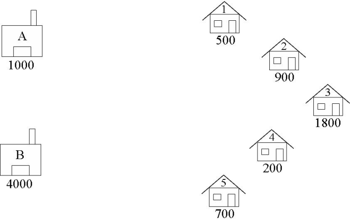
A boutique brewery has two warehouses from which it distributes beer to five carefully chosen bars. At the start of every week, each bar sends an order to the brewery’s head office for so many crates of beer, which is then dispatched from the appropriate warehouse to the bar. The brewery would like to have an interactive computer program which they can run week by week to tell them which warehouse should supply which bar so as to minimize the costs of the whole operation. For example, suppose that at the start of a given week the brewery has 1000 cases at warehouse A, and 4000 cases at warehouse B, and that the bars require 500, 900, 1800, 200, and 700 cases respectively. Which warehouse should supply which bar?
Formulate
For transportation problems, using a graphical representation of the problem is often helpful during formulation. Here is a graphical representation of The Beer Distribution Problem.
####Identify the Decision Variables In transportation problems we are deciding how to transport goods from their supply nodes to their demand nodes. The decision variables are the Arcs connecting these nodes, as shown in the diagram below. We are deciding how many crates of beer to transport from each warehouse to each pub.
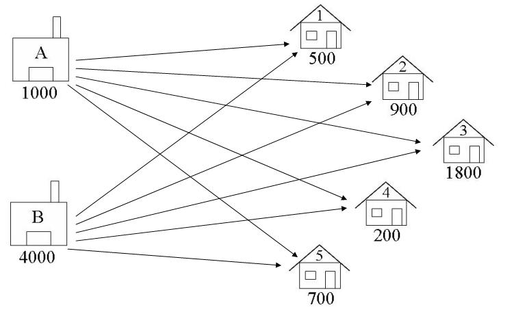
A1 = number of crates of beer to ship from Warehouse A to Bar 1 A5 = number of crates of beer to ship from Warehouse A to Bar 5 B1 = number of crates of beer to ship from Warehouse B to Bar 1 B5 = number of crates of beer to ship from Warehouse B to Bar 5 Let: $\( \begin{align} W &= \{A,B\} \\ B &= \{1, 2, 3, 4, 5 \} \\ x_{(w,b)} &\ge 0 \ldots \forall w \in W, b \in B \\ x_{(w,b)} & \in \mathbb{Z}^+ \ldots \forall w \in W, b \in B \\ \end{align} \)$
The lower bound on the variables is Zero, and the values must all be Integers (since the number of crates cannot be negative or fractional). There is no upper bound.
####Formulate the Objective Function The objective function has been loosely defined as cost. The problem can only be formulated as a linear program if the cost of transportation from warehouse to pub is a linear function of the amounts of crates transported. Note that this is sometimes not the case. This may be due to factors such as economies of scale or fixed costs. For example, transporting 10 crates may not cost 10 times as much as transporting one crate, since it may be the case that one truck can accommodate 10 crates as easily as one. Usually in this situation there are fixed costs in operating a truck which implies that the costs go up in jumps (when an extra truck is required). In these situations, it is possible to model such a cost by using zero-one integer variables: we will look at this later in the course.
We shall assume then that there is a fixed transportation cost per crate. (If the capacity of a truck is small compared with the number of crates that must be delivered then this is a valid assumption). Lets assume we talk with the financial manager, and she gives us the following transportation costs (dollars per crate):
From Warehouse to Bar A B
1 |
2 |
3 |
|---|---|---|
2 |
4 |
1 |
3 |
5 |
3 |
4 |
2 |
2 |
5 |
1 |
3 |
Minimise the Transporting Costs = Cost per crate for RouteA1 * A1 (number of crates on RouteA1)
… + Cost per crate for RouteB5 * B5 (number of crates on RouteB5) \(\min \sum_{w \in W, b \in B} c_{(w,b)} x_{(w,b)}\)
Formulate the Constraints
The constraints come from considerations of supply and demand. The supply of beer at warehouse A is 1000 cases. The total amount of beer shipped from warehouse A cannot exceed this amount. Similarly, the amount of beer shipped from warehouse B cannot exceed the supply of beer at warehouse B. The sum of the values on all the arcs leading out of a warehouse, must be less than or equal to the supply value at that warehouse:
Such that: $\( A_1 + A_2 + A_3 + A_4 + A_5 \leq 1000\\ B_1 + B_2 + B_3 + B_4 + B_5 \leq 4000\\ \sum_{ b \in B} x_{(w,b)} \leq s_w \ldots \forall w \in W \)\( The demand for beer at bar 1 is 500 cases, so the amount of beer delivered there must be at least 500 to avoid lost sales. Similarly, considering the amounts delivered to the other bars must be at least equal to the demand at those bars. Note, we are assuming there are no penalties for oversupplying bars (other than the extra transportation cost we incur). We can _balance_ the transportation problem to make sure that demand is met exactly - there will be more on this later. For now, the sum of the values on all the arcs leading into a bar, must be greater than or equal to the demand value at that bar: \)\( A_1 + B_1 \geq 500\\ A_2 + B_2 \geq 900\\ A_3 + B_3 \geq 1800\\ A_4 + B_4 \geq 200\\ A_5 + B_5 \geq 700\\ \sum_{ w \in W} x_{(w,b)} \geq d_b \ldots \forall b \in B \)$ Finally, we have already specified the amount of beer shipped must be non-negative.
After all this we run it through our code and solve it
!pip install pulp
Collecting pulp
  Downloading PuLP-2.5.1-py3-none-any.whl (41.2 MB)
     |████████████████████████████████| 41.2 MB 1.3 MB/s
?25hInstalling collected packages: pulp
Successfully installed pulp-2.5.1
"""
The Beer Distribution Problem for the PuLP Modeller

Authors: Antony Phillips, Dr Stuart Mitchell    2007
"""

# Import PuLP modeller functions
from pulp import *

# Creates a list of all the supply nodes
Warehouses = ["A","B"]

# Creates a dictionary for the number of units of supply for each supply node
supply = {"A": 1000,
        "B": 4000}

# Creates a list of all demand nodes
Bars = ["1", "2", "3", "4", "5"]

# Creates a dictionary for the number of units of demand for each demand node
demand = {"1": 500,
        "2": 900,
        "3": 1800,
        "4": 200,
        "5": 700}

# Creates a list of costs of each transportation path
costs = {'A': {'1':2,'2':4,'3':5,'4':2,'5':1},
          'B': {'1':3,'2':1,'3':3,'4':2,'5':3}}


# Creates the prob variable to contain the problem data
prob = LpProblem("Beer Distribution Problem",LpMinimize)

# Creates a list of tuples containing all the possible routes for transport
Routes = [(w,b) for w in Warehouses for b in Bars]

# A dictionary called route_vars is created to contain the referenced variables (the routes)
route_vars = LpVariable.dicts("Route",(Warehouses,Bars),0,None,LpInteger)

# The objective function is added to prob first
prob += lpSum([route_vars[w][b]*costs[w][b] for (w,b) in Routes]), "Sum of Transporting Costs"

# The supply maximum constraints are added to prob for each supply node (warehouse)
for w in Warehouses:
    prob += lpSum([route_vars[w][b] for b in Bars]) <= supply[w], "Sum of Products out of Warehouse %s"%w
    print(prob)

# The demand minimum constraints are added to prob for each demand node (bar)
for b in Bars:
    prob += lpSum([route_vars[w][b] for w in Warehouses]) >= demand[b], "Sum of Products into Bars %s"%b
    print(prob)
Beer_Distribution_Problem:
MINIMIZE
2*Route_A_1 + 4*Route_A_2 + 5*Route_A_3 + 2*Route_A_4 + 1*Route_A_5 + 3*Route_B_1 + 1*Route_B_2 + 3*Route_B_3 + 2*Route_B_4 + 3*Route_B_5 + 0
SUBJECT TO
Sum_of_Products_out_of_Warehouse_A: Route_A_1 + Route_A_2 + Route_A_3
 + Route_A_4 + Route_A_5 <= 1000

VARIABLES
0 <= Route_A_1 Integer
0 <= Route_A_2 Integer
0 <= Route_A_3 Integer
0 <= Route_A_4 Integer
0 <= Route_A_5 Integer
0 <= Route_B_1 Integer
0 <= Route_B_2 Integer
0 <= Route_B_3 Integer
0 <= Route_B_4 Integer
0 <= Route_B_5 Integer

Beer_Distribution_Problem:
MINIMIZE
2*Route_A_1 + 4*Route_A_2 + 5*Route_A_3 + 2*Route_A_4 + 1*Route_A_5 + 3*Route_B_1 + 1*Route_B_2 + 3*Route_B_3 + 2*Route_B_4 + 3*Route_B_5 + 0
SUBJECT TO
Sum_of_Products_out_of_Warehouse_A: Route_A_1 + Route_A_2 + Route_A_3
 + Route_A_4 + Route_A_5 <= 1000

Sum_of_Products_out_of_Warehouse_B: Route_B_1 + Route_B_2 + Route_B_3
 + Route_B_4 + Route_B_5 <= 4000

Sum_of_Products_into_Bars_1: Route_A_1 + Route_B_1 >= 500

Sum_of_Products_into_Bars_2: Route_A_2 + Route_B_2 >= 900

Sum_of_Products_into_Bars_3: Route_A_3 + Route_B_3 >= 1800

Sum_of_Products_into_Bars_4: Route_A_4 + Route_B_4 >= 200

Sum_of_Products_into_Bars_5: Route_A_5 + Route_B_5 >= 700

VARIABLES
0 <= Route_A_1 Integer
0 <= Route_A_2 Integer
0 <= Route_A_3 Integer
0 <= Route_A_4 Integer
0 <= Route_A_5 Integer
0 <= Route_B_1 Integer
0 <= Route_B_2 Integer
0 <= Route_B_3 Integer
0 <= Route_B_4 Integer
0 <= Route_B_5 Integer
/usr/local/lib/python3.7/dist-packages/pulp/pulp.py:1313: UserWarning: Spaces are not permitted in the name. Converted to '_'
  warnings.warn("Spaces are not permitted in the name. Converted to '_'")
References
“The Transportation Problem and the Assignment Problem.” Edited by Ana Zelaia Jauregi, OpenCourseWare, 2012, ocw.ehu.eus/pluginfile.php/40949/mod_resource/content/1/5_Transportation_Exercises.pdf.
Geismar, Niel, et al. “The Integrated Production and Transportation Scheduling Problem for a Product with a Short Lifespan.” INFORMS, vol. 20, no. 1, 2008, pp. 21–33. Winter, doi:10.1287/ijoc.1060.0208.
Coin-or.org. 2021. A Transportation Problem — PuLP v1.4.6 documentation. [online] Available at: https://www.coin-or.org/PuLP/CaseStudies/a_transportation_problem.html [Accessed 27 October 2021].
Taha, H. A. (2017). Chapter 5: Transportation Model and its Varients. In Operations Research An Introduction (Tenth, pp. 179–179). Book, Pearson.
https://cnls.lanl.gov/MK/index.html
https://transportgeography.org/contents/chapter3/provision-and-demand-of-transportation/
Problems
Describe what a node and arc is
Define the main goal of the Optimal Transportation problem
Explain the connection between a node and arc
We have one factory and two warehouses. We have a supply of 25 at the factory. There is also a demand of 15 at warehouse one and a demand of 10. It costs 8 dollars a unit to ship to warehouse one and 13 dollars a unit to ship to warehouse two. Find the optimal solution
We have one factory and two warehouses. We have a supply of 40 at the factory. There is also a demand of 20 at warehouse one and a demand of 16. It costs 9 dollars a unit to ship to warehouse one and 11 dollars a unit to ship to warehouse two. Find the optimal solution
We have one factory and two warehouses. We have a supply of 31 at the factory. There is also a demand of 18 at warehouse one and a demand of 13. It costs 3 dollars a unit to ship to warehouse one and 17 dollars a unit to ship to warehouse two. Find the optimal solution
There are two factories and two warehouses. Factory A and Factory B have 50 and 40 cases each. The demand at Warehouse one is 6 and the demand at warehouse two is 2. The cost to transport from A to one is 6 dollars and to transport from A to two is 5 dollars. The cost to transport from B to One is 4 dollars and the cost to transport from B to two is 7 dollars. Find the optimal solution.
There are two factories and two warehouses. Factory A and Factory B have 90 and 60 cases each. The demand at Warehouse one is 7 and the demand at warehouse two is 9. The cost to transport from A to one is 10 dollars and to transport from A to two is 2 dollars. The cost to transport from B to One is 4 dollars and the cost to transport from B to two is 6 dollars. Find the optimal solution.
There are two factories and three warehouses. With factory A and factory B we have 20 and 40 cases respectively. The demand at warehouse one is 7, warehouse two is 3, and warehouse three is 4. It costs 13 dollars to ship from A to one, 4 dollars to ship from A to two, and 8 dollars to ship from A to three. It costs 8 dollars to ship from B to 1, 4 dollars to ship from B to two, and 13 dollars to ship from B to 3. Find the optimal solution
There are two factories and two warehouses. Factory A and Factory B have 30 and 20 cases each. The demand at Warehouse one is 1 and the demand at warehouse two is 9. The cost to transport from A to one is 11 dollars and to transport from A to two is 6 dollars. The cost to transport from B to One is 7 dollars and the cost to transport from B to two is 13 dollars. Find the optimal solution.
Project Idea
Let us look at another example. This time lets take three factories and three warehouses. It costs a certain amount to ship from a factory to a warehouse. It costs 4 dollars to ship from factory 1 to Warehouse 1. It costs 3 dollars to ship from factory 1 to Warehouse 2. It costs 8 dollars to ship from factory 1 to warehouse 3. The supply of factory 1 is 300 units. From factory 2 it costs 7 dollars to ship to warehouse 1, 5 dollars to ship to warehouse 2, and 9 dollars to ship to warehouse 3. The supply for factory 2 is 300 units. From factory 3 it costs 4 dollars to ship to warehouse 1, 5 dollars to ship to warehouse 2, and 5 dollars to ship to warehouse 3. The supply from factory 3 is 100 units. The demand for warehouse 1 is 200 units, the demand for warehouse 2 is 200 units, and the demand for warehouse 3 is 300.
Take two bags of candy and get 3 destinations to take said candy. Each destination will demand a certain amount of candy. It will cost a certain amount to deliver the candy. The idea is to visualize what is happening in the supply and demand chain. Optimizing how each candy is delivered.