Network Model¶

Introduction¶

Many problems in computer science can be presented in the form of graphs which consists of nodes & links between them. Network flow problems can be taken as an example, as it involves the transportation of goods and material across networks. The motivation for taking advantage of their structure usually has been the need to solve larger problems than otherwise would be possible to solve with existing computer technology. Historically, the first of these special structures to be analyzed was the transportation problem, which is a particular type of network problem. The development of an efficient solution procedure for this problem resulted in the first widespread application of linear programming to problems of industrial logistics. More recently, the development of algorithms to efficiently solve particular large-scale systems has become a major concern in applied mathematical programming.

History Of Network Model¶

It was introduced by Charles Bachaman and developed into standard specifications by Conference on Data System Language (CODASYL) Consortium in 1969.Researchers sponsered by the U.S. Department of Defensen’s Advanced Researvh Projects Agency created the First Packet-switched network, called the ARPANET, in 1969.

Today’s globalization as the world has evolved to an advanced planet in Information Technology because of computer networks. One of the key contributing factors of the information technology rise in the world is network and data communication because of network and technology’s advancement as the system. The goal of network model has always been same, which is convergence and achieving service integration. From early 1960s to present, the development and progress that network model has gone through has always accommodated the rapidly increasing number of users and applications. It has made the global environment of information and technology transparent to applications.

Example 1¶

Shortest Route/Path Problem¶

In Network Models, problems can be presented in many ways. Here, one of the common problem is the shortest route problems. Shortest route problem is a network model problem which has received a great deal of attention for both the practical and theoretical reasons. For instance, given a network with a distance associated with each arc, this network model helps us to find the shortest distance from origin (source) to the destination (which is called sink).

These problems can be formulated in real life problems like equipment replacement, capital, investment, project scheduling, and inventory planning. The theoretical interest of this problem is due to the efficient solution problems. Shortest route problems can be interpreted as a network problem very easily.

A graph’s shortest route issue asks for a path between vertices that has the least total weight of all its edges [5-7]. In which we must identify all the paths and then we must sum of all the distances of specific path. Then the path has less distance it will be considered as the shortest route.

Example¶

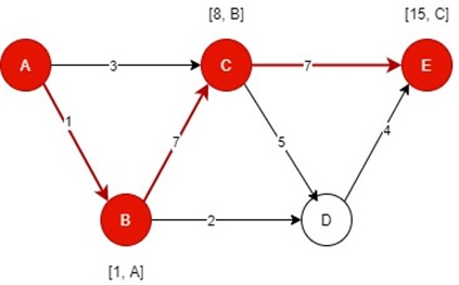
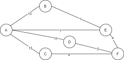
Find the shortest path in the given graph from point A to E.

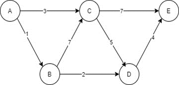
It’s a directed graph firstly we will see all possible path in it. So, the possible paths are:

Path no.	Path
1	A-C-E
2	A-C-D-E
3	A-B-C-E
4	A-B-C-D-E
5	A-B-D-E

After executing the whole path, we will calculate the distance of every node included in the selected path then the path has overall less distance will be the shortest path.

Path 1:

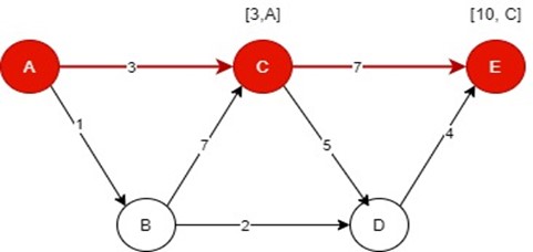
In the bracket [m, n] m is basically distance between two nodes and the n is parent node from which we are coming from. So, as above 3 is distance between A to C which is m and, C parent node is A which is n. So, the distance of path 1 is 10

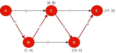
Path 2:

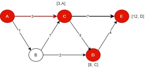
The distance of path 2 is 12

Path 3:

The distance of path 3 is 15

Path 4:

The distance of path 4 is 17

Path 5:

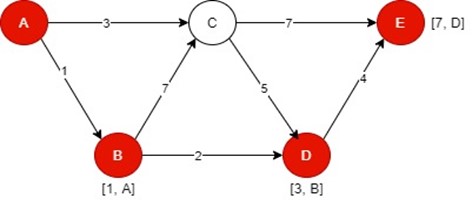
The distance of path 5 is 7.

So, the results are in the given table:

Path no.	Path	Distance
1	A-C-E	10
2	A-C-D-E	12
3	A-B-C-E	15
4	A-B-C-D-E	17
5	A-B-D-E	7

So, the shortest path is path 5 which is A-B-D-E with distance 7.

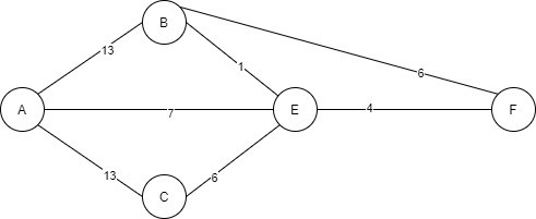
Solving Example 1 to find shortest path using python¶

#Solving Example 1 to find the Shortest path using python...

import sys

class Graph():

    def __init__(self, vertices):
        self.V = vertices
        self.graph = [[0 for column in range(vertices)]
                        for row in range(vertices)]

    def printSolution(self, dist):
        print ("The shortest path from A to F is:- ")
        print(dist[self.V-1])

    #A utility function to find the vertex with
    # minimum distance value, from the set of vertices
    # not yet included in shortest path tree

    def minDistance(self, dist, sptSet):

        # Initialize minimum distance for next node
        min = sys.maxsize


        for u in range(self.V):
            if dist[u] < min and sptSet[u] == False:
                min = dist[u]
                min_index = u

        return min_index

 # Funtion that implements Dijkstra's single source
 # shortest path algorithm for a graph represented
 # using adjacency matrix representation

 # Implementation
    def dijkstra(self, src):
    
        dist = [sys.maxsize] * self.V
        dist[src] = 0
        sptSet = [False] * self.V
    
        for cout in range(self.V):

            x = self.minDistance(dist, sptSet)

            sptSet[x] = True

            for y in range(self.V):
                if self.graph[x][y] > 0 and sptSet[y] == False and dist[y] > dist[x] + self.graph[x][y]:
                        dist[y] = dist[x] + self.graph[x][y]

        self.printSolution(dist)

# Driver program
g = Graph(5)
g.graph = [[0,13,13,7,0],
           [13,0,0,1,6],
           [13,0,0,6,0],
           [7,1,6,0,4],
           [0,6,0,4,0]
           ];

g.dijkstra(0);

The shortest path from A to F is:- 
11

Example 2¶

Maximal Overflow¶

The maximum quantity of flow that can flow from a source to a sink across a network is what this term refers to. The maximum flow problem may be solved using a variety of techniques [1]. Ford-Fulkerson method and Dinic’s Algorithm are two popular solutions methods to this type of problem. Here, we are going to be using Ford-Fulkerson method to solve the problems.

Heres how to implement the problems.¶

DFS or BFS may be used to locate an augmenting path in the residual graph.
The steps involved in updating the residual graph are as follows: (for a better understanding, see the diagrams.)
The minimal capacity in the path is deducted from all the path's edges for each edge in the augmentation path.
For each additional node along the augmenting path, an edge of the same length is added in the reverse direction to the existing edges. Since the path from the source to the sink determines the algorithm’s complexity, it can’t be calculated with precision.

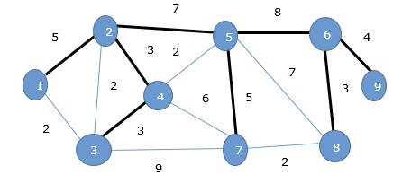
Example¶

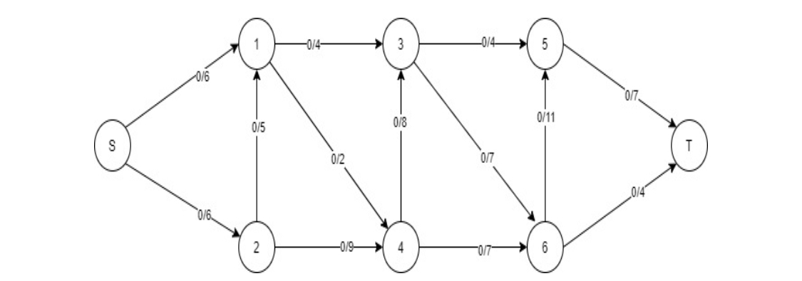
Find the Max flow for the given graph G from the source S to destination T.

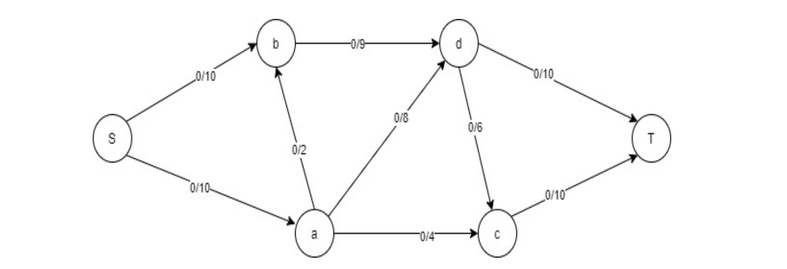
**Path 1:**Set the edge flow to 0 on all of them. Find a augmenting path in the residual network that has a higher capacity. In this case, I’m going to choose the S-a-b-d-c-T. A bottleneck capacity is the maximum flow that a route can handle in a certain time. You can see that the bottleneck capacity is 2 along this line. Update the edge flow values in the augmenting path now, but don’t go over the capacity limit. After that, you’ll have the flow network below and the residual network to deal with.

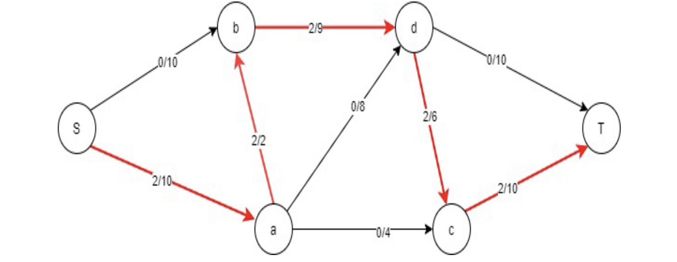
Flow= S-a-b-d-c-T =2

Path 2: Then I select the augmenting path S-a-c–T. Now the bottleneck capacity is 4.

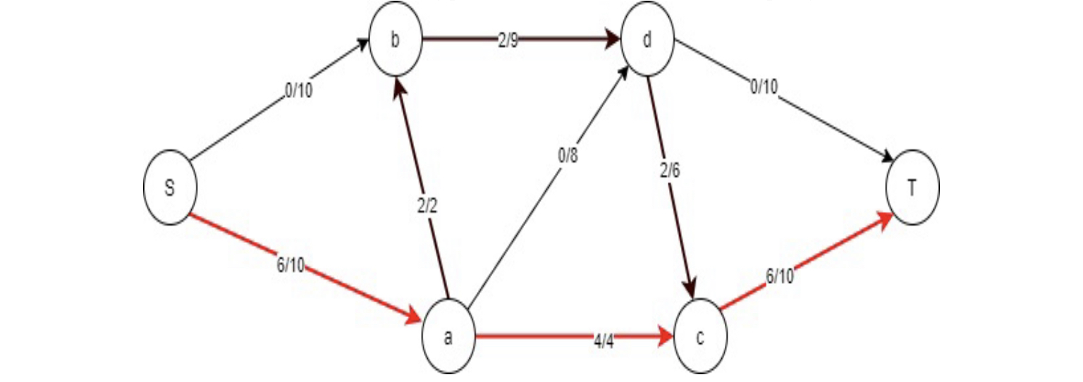
Flow= S-a-c-T = 4

Path 3: Then I select the augmenting path S-a-d-c-T. Now the bottleneck capacity is 4.

Flow= S-a-d-c-T= 4

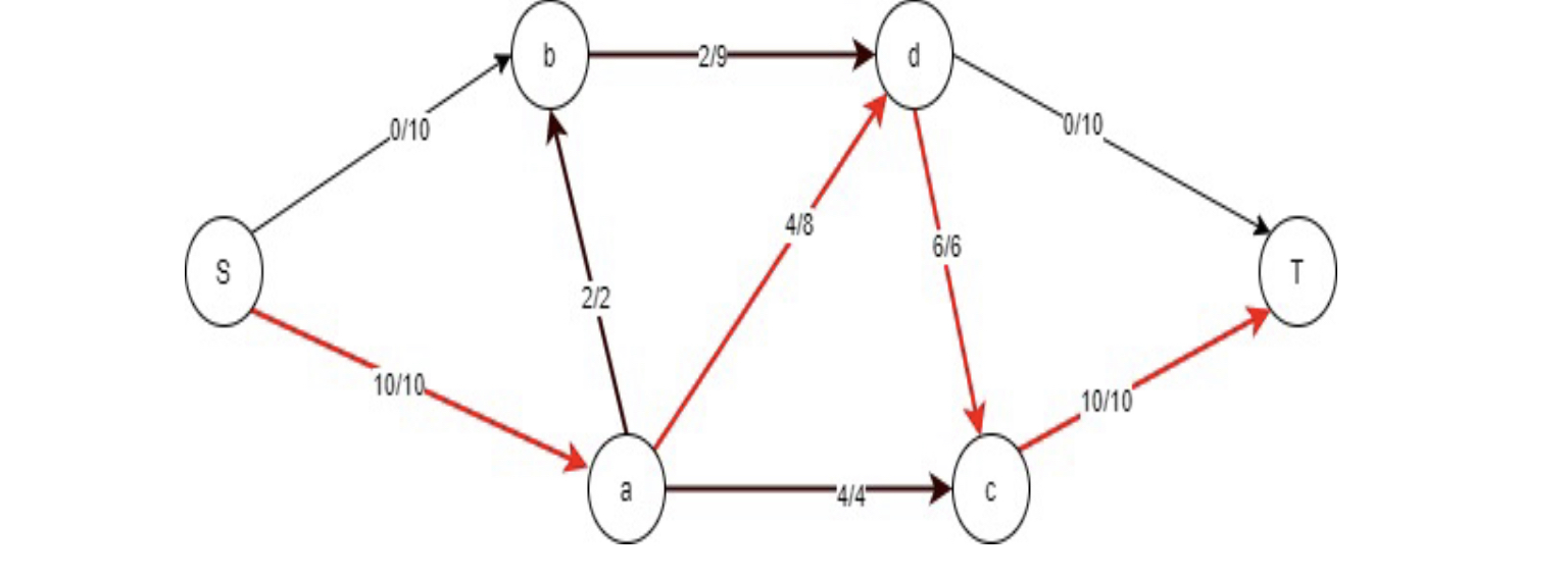
Path 4: Then I select the augmenting path S-b-a-d-T. Reverse flow in it so there is no bottleneck.

Reverse FLOW

Path 5: Then I select the augmenting path S-b-d-T. Now the bottleneck capacity is 9.

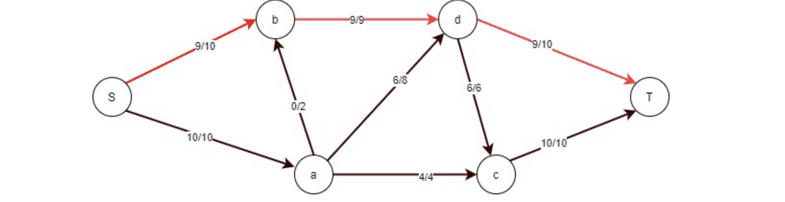
Flow=S-b-d-T= 9
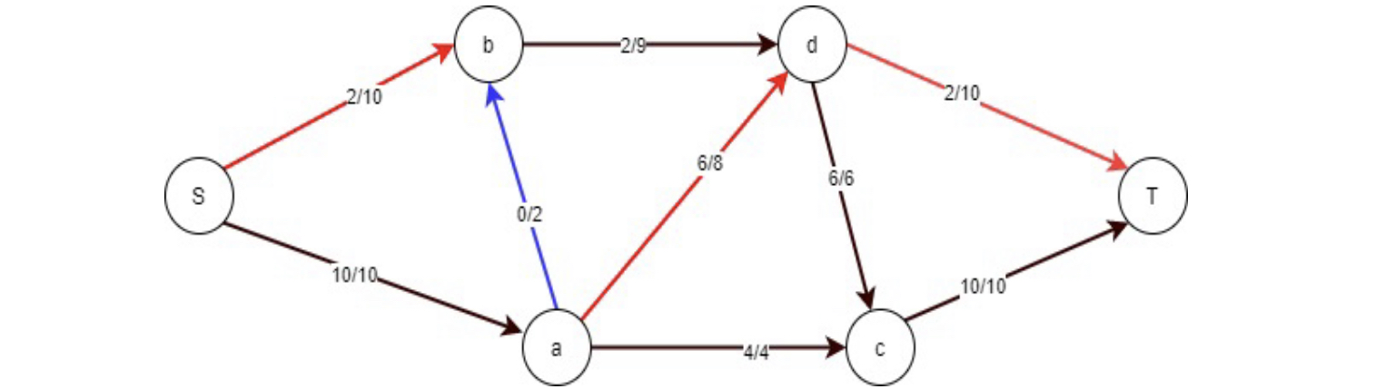
The residual graph is now empty since there are no more routes connecting s and t. As a result, there’s no way to make it flow. The Ford Fulkerson technique is complete, and we can now proceed to finding the highest flow rate possible using this information. The maximum flow is equal to the source flow. And the max flow for this is given below
Max Flow= 2+4+4+9=19

Solving the above Question in example 2 to find maximal flow using python¶

#Solving the above Question in example 2 to find maximal flow using python
#We took the codes as references from different python language sources and encoded in here.

class Graph:
 
    def __init__(self, graph):
        self.graph = graph  # residual graph
        self. ROW = len(graph)

    '''Returns true if there is a path from source 's' to sink 't' in
    residual graph. Also fills parent[] to store the path '''
 
    def BFS(self, s, t, parent):
 
        # Mark all the vertices as not visited
        visited = [False]*(self.ROW)
 
        # Create a queue for BFS
        queue = []
 
        # Mark the source node as visited and enqueue it
        queue.append(s)
        visited[s] = True
 
         # Standard BFS Loop
        while queue:
 
            # Dequeue a vertex from queue and print it
            u = queue.pop(0)
 
          
            for ind, val in enumerate(self.graph[u]):
                if visited[ind] == False and val > 0:
                     
                    queue.append(ind)
                    visited[ind] = True
                    parent[ind] = u
                    if ind == t:
                        return True
 
        
        return False
             
     
    # Returns tne maximum flow from s to t in the given graph
    def FordFulkerson(self, source, sink):
 
        # This array is filled by BFS and to store path
        parent = [-1]*(self.ROW)
 
        max_flow = 0 # There is no flow initially
 
        while self.BFS(source, sink, parent) :
 
        
            path_flow = float("Inf")
            s = sink
            while(s !=  source):
                path_flow = min (path_flow, self.graph[parent[s]][s])
                s = parent[s]
 
            # Add path flow to overall flow
            max_flow +=  path_flow
 
            # update residual capacities of the edges and reverse edges
            # along the path
            v = sink
            while(v !=  source):
                u = parent[v]
                self.graph[u][v] -= path_flow
                self.graph[v][u] += path_flow
                v = parent[v]
 
        return max_flow
graph = [[0, 10, 10, 0, 0, 0],
        [0, 0, 2, 4, 8, 0],
        [0, 0, 0, 0, 9, 0],
        [0, 0, 0, 0, 0, 10],
        [0, 0, 0, 6, 0, 10],
        [0, 0, 0, 0, 0, 0]]
 
g = Graph(graph)
 
source = 0; sink = 5
  
print ("The maximum possible flow is %d " % g.FordFulkerson(source, sink))

The maximum possible flow is 19

Example 3¶

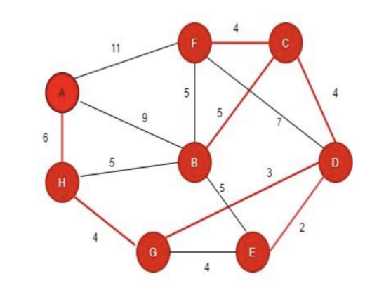
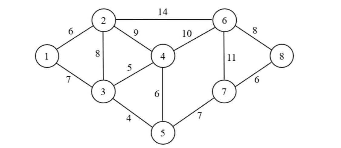
Minimum Spanning Tree¶

Minimizing the lengths (or “weights”) of the edges of a tree is known as a minimal spanning tree [2],[3], [4]. A cable company, for example, could wish to build cable in several areas at the same time. By laying less cable, the cable business saves money.
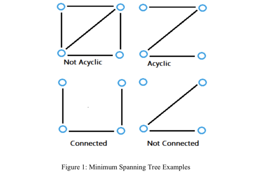
For any pair of vertices in a tree, there is only one path that connects them.
A graph’s spanning tree is one that:

This has all the vertices from the original graph in it.
Extends (spans) to every vertex.
Is an acyclic chain of operations. In other words, the network is devoid of self-referential nodes.

Example¶

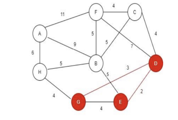
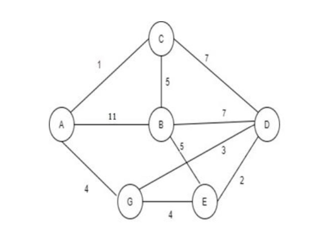
Step 1: Here we are writing the edges that connected with each other and their distance is also mentioned in the table so find the minimum spanning tree for this tree.

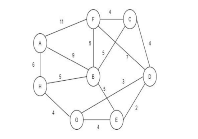
Edge	distance
(D,E)	2
(D,G)	3
(E,G)	4
(C,D)	4
(G,H)	4
(C,F)	4
(B,C)	5
(B,E)	5
(B,F)	5
(B,H)	5
(A,H)	6
(D,F)	7
(A,B)	9
(A,F)	11

**Step 2:**Firstly, we are selecting the edge which has most less distance between the so D to E has less distance that’s why we choose it.

Edge	distance
(D,E)	2	✔
(D,G)	3
(E,G)	4
(C,D)	4
(G,H)	4
(C,F)	4
(B,C)	5
(B,E)	5
(B,F)	5
(B,H)	5
(A,H)	6
(D,F)	7
(A,B)	9
(A,F)	11

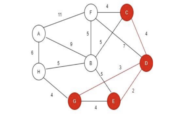
**Step 3:**Now, select the node that is connected to D or E with with the less distance as we see in the tree D to G is 3 which is less distance among all the nodes connected with the D and E. Also adding their entry in the table.

Edge	distance
(D,E)	2	✔
(D,G)	3	✔
(E,G)	4
(C,D)	4
(G,H)	4
(C,F)	4
(B,C)	5
(B,E)	5
(B,F)	5
(B,H)	5
(A,H)	6
(D,F)	7
(A,B)	9
(A,F)	11

**Step 4:**Now here we are also searching for the node that has least distance among all the nodes connected to D, E, and G.

Edge	distance
(D,E)	2	✔
(D,G)	3	✔
(E,G)	4	✖
(E,G)	4	✔
(C,D)	4
(G,H)	4
(C,F)	4
(B,C)	5
(B,E)	5
(B,F)	5
(B,H)	5
(A,H)	6
(D,F)	7
(A,B)	9
(A,F)	11

Step 5: Searching for the node that has least distance among all the nodes connected to D, E, C and G.

Edge	distance
(D,E)	2	✔
(D,G)	3	✔
(E,G)	4	✖
(C,D)	4	✔
(G,H)	4	✔
(C,F)	4
(B,C)	5
(B,E)	5
(B,F)	5
(B,H)	5
(A,H)	6
(D,F)	7
(A,B)	9
(A,F)	11

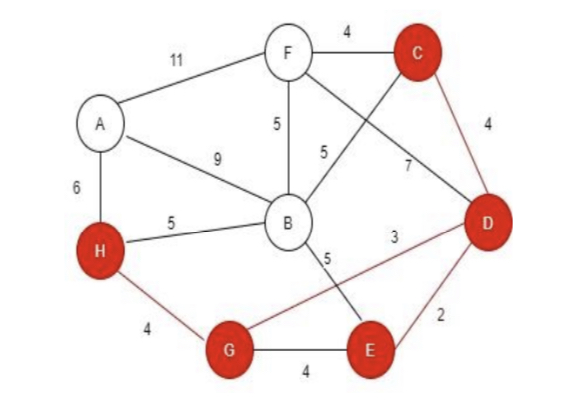
Step 6: Searching for the node that has least distance among all the nodes connected to D, E, C, H and G.

Edge	distance
(D,E)	2	✔
(D,G)	3	✔
(E,G)	4	✖
(C,D)	4	✔
(G,H)	4	✔
(C,F)	4	✔
(B,C)	5
(B,E)	5
(B,F)	5
(B,H)	5
(A,H)	6
(D,F)	7
(A,B)	9
(A,F)	11

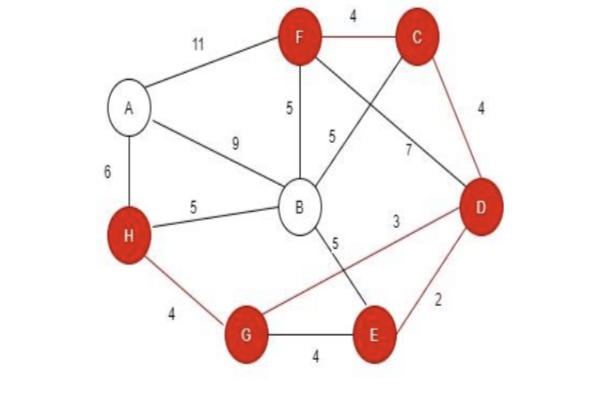
Step 7: Searching for the node that has least distance among all the nodes connected to D, E, C, H, F and G.

Edge	distance
(D,E)	2	✔
(D,G)	3	✔
(E,G)	4	✖
(C,D)	4	✔
(G,H)	4	✔
(C,F)	4	✔
(B,C)	5	✔
(B,E)	5
(B,F)	5
(B,H)	5
(A,H)	6
(D,F)	7
(A,B)	9
(A,F)	11

Step 8: Searching for the node that has least distance among all the nodes connected to D, E, C, H, F, B and G.

Edge	distance
(D,E)	2	✔
(D,G)	3	✔
(E,G)	4	✖
(C,D)	4	✔
(G,H)	4	✔
(C,F)	4	✔
(B,C)	5	✔
(B,E)	5	✖
(B,F)	5	✖
(B,H)	5	✖
(A,H)	6	✔
(D,F)	7
(A,B)	9
(A,F)	11

Step 9: So here we discover all the nodes and discovered all these through visiting the path with smallest distance and we can’t make a cycle in it and cant visit the node twice.

Edge	distance
(D,E)	2	✔
(D,G)	3	✔
(E,G)	4	✖
(C,D)	4	✔
(G,H)	4	✔
(C,F)	4	✔
(B,C)	5	✔
(B,E)	5	✖
(B,F)	5	✖
(B,H)	5	✖
(A,H)	6	✔
(D,F)	7	-
(A,B)	9	-
(A,F)	11	-

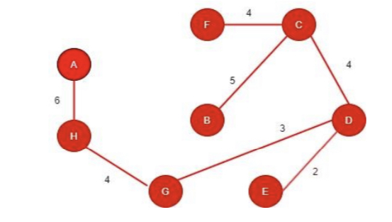
So, the total cost we got = 28

Solving the above Question in example 3 for Minimum spanning tree using python¶

#Solving the above Question in example 3 to solve Minimum spanning tree using python
#We took the codes as references from different python language sources.

# to do union by rank of x and y
def union(parent, rank, x, y):
    xparent = find(parent, x)
    yparent = find(parent, y)

    if rank[xparent] < rank[yparent]:
        parent[xparent] = yparent
    elif rank[xparent] > rank[yparent]:
        parent[yparent] = xparent
    else:
        parent[yparent] = xparent
        rank[xparent] += 1

# Function to find parent of X Uses path compression technique
def find(parent, x):
        if parent[x] == x:
                return x
        return find(parent, parent[x])

def mst(graph, V, E):
        # to keep track for vertices covered
        e = 0
        # to keep track of newly added edges into MST
        k = 0

        # to store the parent of each node
        parent=[]

        # to store rank of
        rank = []
        for vertex in range(V):
                parent.append(vertex)
                rank.append(0)

        result = []
        # Total Number of edges going into mst are 1 Less then number of vertices
        while e < V - 1:
                # Selecting the edge having smallest weight
                v1, v2, w = graph[k]
                k = k + 1
                x = find(parent, v1)
                y = find(parent, v2)
                print(x,y)
                # Checking if including this edge creates a cycle
                if x != y:
                        e = e + 1
                        result.append([v1, v2, w])
                        union(parent, rank, x, y)
                # if v1 and v2 hav the same parent which is x==y ignore the edge

                minimumCost = 0
                print ("Edges in the constructed MST")
                for u, v, weight in result:
                        minimumCost += weight
                        print("%d -- %d == %d" % (u, v, weight))
                print("Minimum Spanning Tree" , minimumCost)


# Creating A Graph
graph = []
no_of_Vertices = 6
no_of_Edges = 10

graph.append([0,1,11])
graph.append([0,2,1])
graph.append([1,2,5])
graph.append([1,3,7])
graph.append([2,3,7])
graph.append([1,4,5])
graph.append([3,4,2])
graph.append([3,5,3])
graph.append([4,5,4])
graph.append([0,5,4])


# Code for taking Input From user
# for i in range(no_of_Edges):
#       print("Enter Vertex1, Vertex2, Weight space separated\n")
#       v1,v2,w = input().strip().split(" ")
#       graph.append([int(v1),int(v2),int(w)])

# Sort the graph according to Edge weights
graph = sorted(graph,key=lambda x: x[2])
# Calling Minimum Spanning Tree Function
mst(graph,no_of_Vertices,no_of_Edges)

0 2
Edges in the constructed MST
0 -- 2 == 1
Minimum Spanning Tree 1
3 4
Edges in the constructed MST
0 -- 2 == 1
3 -- 4 == 2
Minimum Spanning Tree 3
3 5
Edges in the constructed MST
0 -- 2 == 1
3 -- 4 == 2
3 -- 5 == 3
Minimum Spanning Tree 6
3 3
Edges in the constructed MST
0 -- 2 == 1
3 -- 4 == 2
3 -- 5 == 3
Minimum Spanning Tree 6
0 3
Edges in the constructed MST
0 -- 2 == 1
3 -- 4 == 2
3 -- 5 == 3
0 -- 5 == 4
Minimum Spanning Tree 10
1 0
Edges in the constructed MST
0 -- 2 == 1
3 -- 4 == 2
3 -- 5 == 3
0 -- 5 == 4
1 -- 2 == 5
Minimum Spanning Tree 15

Problems¶

Question 1¶

Find the shortest path from the given graph from point A to E.

Question 2¶

Find the shortest path from the given graph from point A to F.

Question 3¶

Find the shortest path from the given graph from point A to F.

Question 4¶

Find the Max flow for the given graph G from the source S to destination T.

Question 5¶

Find the Max flow for the given graph G from the source S to destination T.

Question 6¶

Find the Max flow for the given graph G from the source S to destination T.

Question 7¶

Find the Minimum Spanning Tree of the following from point A to G.

Question 8¶

Find the Minimum Spanning Tree of the following from point A to H.

Question 9¶

Find the Minimum Spanning Tree of the following network from point 1 to 8.

Question 10¶

Find the Minimum Spanning Tree of the following from poinnt 1 to 9.

Project Ideas¶

Network model is such a huge topic, it pretty much covers every concepts within the information and technology. One of the reasons why one must understand the concept of network model is because it helps to break down larger problems into smallers ones and split them into chunks so that they can be easilt managed. They represent a framework for dividing up the tasks needed to implement a network. The basic features of network model, such as optimization and modularity, has always been a boon for large scale industries to small businessess which as continuouly helped them enhance and modify systems for a common cause.

Overall, we were so fascinated by this topic and the idea of network science, we wanted to explore the diversity, history and culture of this model. This really got us going.

References¶

Bradley, Hax, and Magnanti. Network Models. Applied Mathematical Programming. Addison – Wesley, 1977. http://web.mit.edu/15.053/www/AMP.htm. Accessed 16 Sep 2021.
Barua, Saurav. (2019). Operation Research Problems Solving in Python. 10.13140/RG.2.2.20719.38565. https://www.researchgate.net/publication/335572221_Operation_Research_Problems_Solving_in_Python. Accessed 18 Sep 2021.
Taha, H. A. (2017). Network Model). In Operations research: An introduction (10th ed.). pp. 220, 225, 235, Pearson. Accessed 19 Sept 2021.
L. R. Ford and D. R. Fulkerson, “Maximal Flow Through a Network,” Canadian Journal of Mathematics, vol. 8, pp. 399–404, 1956, doi: 10.4153/cjm-1956-045-5. Accessed 20 Oct 2021.
A. Kershenbaum, “Computing capacitated minimal spanning trees efficiently,” Networks, vol. 4, no. 4, pp. 299–310, 1974, doi: 10.1002/net.3230040403. Accessed 18 Oct 2021.
T. C. Hu, “Optimum Communication Spanning Trees,” SIAM Journal on Computing, vol. 3, no. 3, pp. 188–195, Sep. 1974, doi: 10.1137/0203015. Accessed 18 Sep 2021.
A. A. and N. Eckson, “Robust Water Distribution System using Minimal Spanning Tree Algorithm,” International Journal of Computer Applications, vol. 158, no. 1, pp. 1–4, Jan. 2017, doi: 10.5120/ijca2017912724. Accessed 18 Oct 2021.
A. Fitro, S. Suryono, and R. Kusumaningrum, “Shortest Route at Dynamic Location with Node Combination-Dijkstra Algorithm,” Proceeding of the Electrical Engineering Computer Science and Informatics, vol. 5, no. 1, Nov. 2018, doi: 10.11591/eecsi.v5.1604. Accessed 18 Oct 2021.
Bing Liu et al., “Finding the shortest route using cases, knowledge, and Djikstra’s algorithm,” IEEE Expert, vol. 9, no. 5, pp. 7–11, Oct. 1994, doi: 10.1109/64.331478. Accessed 18 Oct 2021.
J. Wang and T. Kaempke, “Shortest route computation in distributed systems,” Computers & Operations Research, vol. 31, no. 10, pp. 1621–1633, Sep. 2004, doi: 10.1016/s0305-0548(03)00111-4. Accessed 9 Oct 2021.

Authors¶

Principal author of this chapter were: Sachin Samal, Prakash Silwal, Watan Chaudhary

Contributions were also made by: Dr. Nicholas Jacob

Operations Research OER

Network Model¶

Introduction¶

History Of Network Model¶

Example 1¶

Shortest Route/Path Problem¶

Example¶

Solving Example 1 to find shortest path using python¶

Example 2¶

Maximal Overflow¶

Heres how to implement the problems.¶

Example¶

Solving the above Question in example 2 to find maximal flow using python¶

Example 3¶

Minimum Spanning Tree¶

Example¶

Solving the above Question in example 3 for Minimum spanning tree using python¶

Problems¶

Question 1¶

Question 2¶

Question 3¶

Question 4¶

Question 5¶

Question 6¶

Question 7¶

Question 8¶

Question 9¶

Question 10¶

Project Ideas¶

References¶

Authors¶