Gradient Descent
Introduction
Gradient descent is an optimization aglorithm that is used for one thing: finding the local minimum of the differentiable function. How we are able to find that is once we find a spot of the function’s gradient, we need to repeat the steps until we eventually get to the functions local minumum.
This algorithm was first introduced to the world by Augustin-Louis Cauchy back in the year of 1847. He created this algorithm to help solve larger optimization problems in a short amount of time that were used in studying astrology. Although it’s still used in astrology today, we also use it in our daily live’s without realizing that we are using gradient descent.
For example, when students are going to class we need to find the quickest way to class. Also when we are driving, we are wanting to get to our desination the quickest so we can save our time and gas. When it comes to making huge purchases in life, like a vehicle. Once we know what vehicle that we want to purchase, we usually travel to different dealerships to find that vehicle with the cheapest price.

Figure 1: Visualization of gradient descent
Theory of Gradient Descent
While gradient descent is the main section that we will be talking about in this section,there are different types of gradient descent. There’s three types of algorithms: batch, socratic, and mini-batch gradient descent. While these are all of the gradient descent algorithm categories,they are used for different categories.
Batch Gradient Descent - It calculates the error of each example in the dataset but only after all of the training values have been evaluated and the model has been upgraded. This type is great for producing a stable error and convergience.
Socratic Gradient Descent - This is used within the dataset. In other words, its updates the parameters for each example one-by-one. Depending on the problem, socratic gradient descent can be quicker than the batch.
Mini-Batch Gradient Descent - This version is a mixture of both batch and socratic gradient descent. It is the go-to method because it simply splits the training data into small batches and performs an update for every batch. This type is the most common type of gradient descent.
When it comes to finding the gradient descent of a function, we need to understand what we are trying to find. When you try to calculate the gradient descent, the student needs to follow the negative slope of the objective function in order to locate the minimum of the function. The minimum is also known as the cost.
When it’s a positive slope then it’s a minimum, when it’s a negative slope, then it’s the maximum.
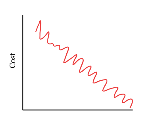
Figure 2: Mini-batch gradient descent
Mountain climbing visualization
Let’s say that someone is trying to walk down a mountain the quickest way possible. The person can’t go straight down because that’s impossible. In order to get to the bottom, we need to take different stops to get to the bottom. The figure below shows a visualization of the statement above.
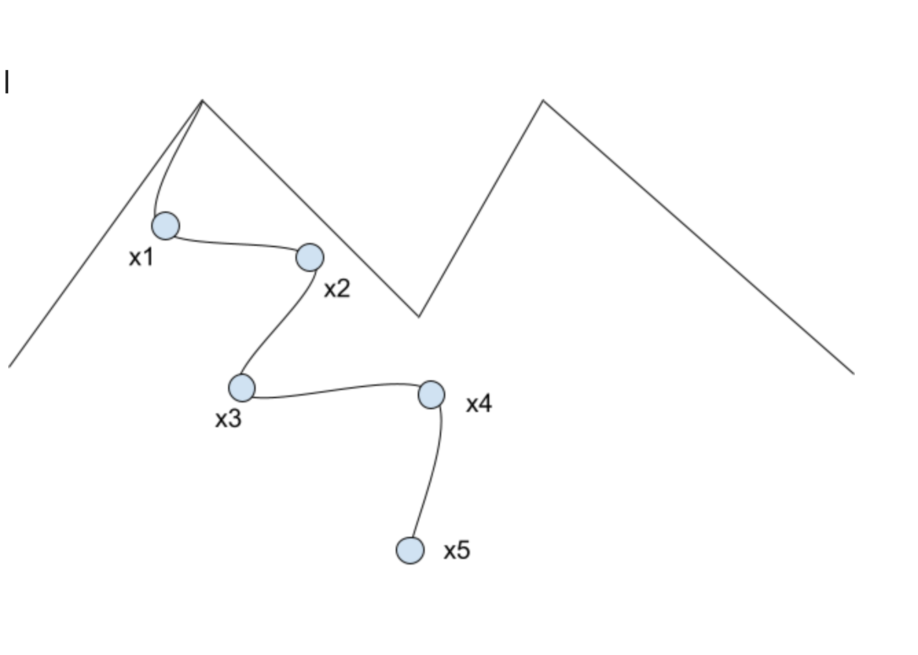
Figure 3: Mountain visualization
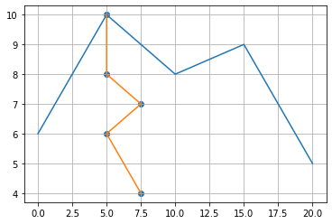
Below is an example is the pseducode of the mountain example:
import matplotlib.pyplot as plt

# x and y coordinates of the mountain
mountain_x=[0,5,10,15,20]
mountain_y=[6,10,8,9,5]

# x and y stop coordinates
stop_x=[5,5,7.5,5,7.5]
stop_y=[10,8,7,6,4]

#plotting the mountain, stops, and path
plt.plot(mountain_x,mountain_y)
plt.scatter(stop_x,stop_y)
plt.plot(stop_x,stop_y)

#visualize the grid
plt.grid()
Here, consider the loss_function() which is a global minimum (x1) and several local minima.
Theory of Gradient Descent
While gradient descent is the main section that we will be talking about in this section,there are different types of gradient descent. There’s three types of algorithms: batch, socratic, and mini-batch gradient descent. While these are all of the gradient descent algorithm categories,they are used for different categories.
Batch Gradient Descent - It calculates the error of each example in the dataset but only after all of the training values have been evaluated and the model has been upgraded. This type is great for producing a stable error and convergience.
Socratic Gradient Descent - This is used within the dataset. In other words, its updates the parameters for each example one-by-one. Depending on the problem, socratic gradient descent can be quicker than the batch.
Mini-Batch Gradient Descent - This version is a mixture of both batch and socratic gradient descent. It is the go-to method because it simply splits the training data into small batches and performs an update for every batch. This type is the most common type of gradient descent.
When it comes to finding the gradient descent of a function, we need to understand what we are trying to find. When you try to calculate the gradient descent, the student needs to follow the negative slope of the objective function in order to locate the minimum of the function. The minimum is also known as the cost.
When it’s a positive slope then it’s a minimum, when it’s a negative slope, then it’s the maximum.
Figure 2: Mini-batch gradient descent
Mountain climbing visualization
Let’s say that someone is trying to walk down a mountain the quickest way possible. The person can’t go straight down because that’s impossible. In order to get to the bottom, we need to take different stops to get to the bottom. The figure below shows a visualization of the statement above.
Figure 3: Mountain visualization
Below is an example is the pseducode of the mountain example:
import matplotlib.pyplot as plt
# x and y coordinates of the mountain
mountain_x=[0,5,10,15,20]
mountain_y=[6,10,8,9,5]
# x and y stop coordinates
stop_x=[5,5,7.5,5,7.5]
stop_y=[10,8,7,6,4]
#plotting the mountain, stops, and path
plt.plot(mountain_x,mountain_y)
plt.scatter(stop_x,stop_y)
plt.plot(stop_x,stop_y)
#visualize the grid
plt.grid()
Here, consider the loss_function() which is a global minimum (x1) and several local minima.
Finding the Gradient Descent in more detail
Below we have an example that goes more indepth with the gradient descent algorithm
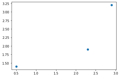
Let’s say that we are trying to find someone peoples weight and height. Here are the following x is the weight and y is the height.
1.(0.5 , 1.4)
2.(2.3 , 1.9)
3.(2.9 ,3.2)
#@title Graph that Shows the Above Points
import matplotlib.pyplot as plt
import numpy as np

xpoints = np.array([0.5 , 2.3 , 2.9])
ypoints = np.array([1.4 , 1.9 , 3.2])

plt.plot(xpoints, ypoints, 'o')
plt.show()
With this algorithm we are able to predict their height with a simple equation:
Predicted Height = intercept + slope x weight
To solve the problem we should do the following:
Start by using GD to find the intercept.
Then we will use GD to solve the Intercept and the Slope.
We plug can plug any number in the Least Squares section. We chose 0.64.
Since we need to find the intercept, pick any number for the intercept and plug it in (for this example, let’s pick 0).
We need to plug in the x-value into the weight function.
When we complete those steps, our equation should look like and we can find the Predicted Height:
Predicted Height = 0 + 0.64 * 0.5
Once we got the Predicted Height, we need to calculate the difference between the Observed and Predicted Height. The Observed Height is the y value of the coordinates of the points from above.
When we find the Predicted Height, we can now find the differences between all of the Observed and Predicted Height. The Observed Height is the y-value.
When we find all of the Predicted Heights, we can finally find the Sum of the Squared Residuals.
We find this by squaring the Sum of the Squared Residuals.
NOTE: We can now plug in any value for the Intercept and get a new Predicted Height
The example below shows where you should plug the number to solve to get the next answer:
For the next person it’ll be:
(1.9 - (intercept + 0.64 x 2.3))^2
The last persons equation will be:
(3.2 - (intercept + 0.64 x 2.9))^2
We now have an equation for the curve and we will need to find the derivative of the function.
Now we need to find the derivative of the sum of the squared residuals.
The equation that we use is:
(d/d intercept) Sum of squared residuals
We need to apply the change rule, once we do that, we will get the following:
-2(1.4-Intercept+0.64x0.5)+-2(1.9-Intercept+0.64x2.3))+-2(3.2-Intercept+0.64x2.9))
Now gradient descent will use it to find where the Sum of the Squared Residuals is the lowest.
Since we have the step size, we can calculate a new intercept:
NEW INTERCEPT = OLD INTERCEPT - STEP SIZE
To see how much the residuals shrink when the intercept we need to plug in 0.57 into the chain rule problem above:
STEP SIZE = -2.3 x LEARNING RATE STEP SIZE = -2.3 x 0.1 -> -0.23 NEW INTERCEPT = 0.57 - (-0.23) -> 0.8 NEW INTERCEPT
Now we need to go back to the derivative equation from earlier and plug in the 0.8 now -2(1.4-(0.8+0.64x0.5) + -2(1.9-(0.8+0.64x0.5))+-2(3.2-(0.8+0.64x2.9)) -> -0.9
the new step size is now -0.9 * 0.1 = -0.09 new intercept is 0.89 when we do it again, the new intercept is 0.92
When we do this 6 times, the Gradient Descent for the intercept is 0.95 because the Gradient Descent gets as close to 0 as possible.
Summary:
Take the derivative of the Loss Function for each parameter in it.
Pick random values for the parameters.
Plug the paramenter values into the derivatives, which is the Gradient.
Calculate the Step Sizes: Step Size = Slope * Learning Rate.
Calculate the New Parameters (e.g. intercept): New Parameter = Old Parameter - Step Size.
Go back to step 3 and repeat the Step Size is very small, or when the Maximum Number of Steps is reached.
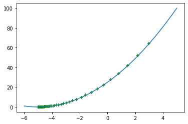
##Find the gradient descent of \(y=(x+5)^2\)
#@title Gradient Descent example graph
import matplotlib.pyplot as plt
import numpy as np

def f(x):
    return (x+5)**2
print(f(5))

def derf(x):
    return 2*(x+5)
i=3
w=0.05
x=i

def gradient_descent(x,weight):
    return x-weight*derf(x)

X=np.arange(-6,5,0.00004)
Y=[f(i) for i in X]

X1=[]

y1=[]

for i in range(100):
    X1.append(x)
    y1.append(f(x))
    x=gradient_descent(x,w)

plt.plot(X,Y)
plt.scatter(X1,y1,marker="+",color="green")
plt.show()
100
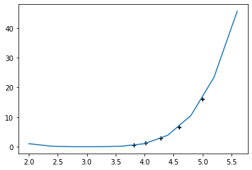
##Example 4
In this example, this is how you’d be able to find the gradient descent using a simple pseudocode to find the local minimum of \(f(x) = (x-3)^4\)
import matplotlib.pyplot as plt
import numpy as np

def f(x):
    return (x-3)**4
print(f(5))

def derf(x):
    return 4*(x-3)
i=5
w=0.05
x=i

def gradient_descent(x,weight):
    return x-weight*derf(x)

X=np.arange(2,6,0.4)
Y=[f(i) for i in X]

X1=[]
y1=[]

for i in range(5):
    X1.append(x)
    y1.append(f(x))
    x=gradient_descent(x,w)

plt.plot(X,Y)
plt.scatter(X1,y1,marker="+",color="black")
plt.show()
16
Problems
Find the gradient descent of \(y=(x+3)^4\)
Explain why gradient descent is important.
How do use gradient descent in our daily lives?
The function is \(y=(9x+2)^2\), what is the gradient descent?
In your own words, describe gradient descent.
Write a simple code to display the gradient descent of \(y=(x+2)^2\)
Find the gradient descent of \(y=(3x-4)^2\)
What is the gradient descent of \(y=(5x-4)^4\)
Find the gradient descent of \(y=(x-5)^2\)
Give an example of the different types of gradient descent.
Conclusion
The gradient descent algorithm is widely used throughout the world. It is used in our daily lives without us realizing what we are using. This algorithm is used to limit the cost of something whether it’s gas being used to get to one place to another. People also use it when they are trying to by a house. For example, they want to purchase a house that has enough square-footage for the best price that is in their budget. Gradient descent is used for nearly anything, this algorithm makes our lives easier.
References
Kumari , Ajitesh “Gradient Descent Explained Simply with Examples.” Data Analytics, https://vitalflux.com/gradient-descent-explained-simply-with-examples/.
Starmer, Josh Gradient Descent, Step-by-Step - Youtube. https://www.youtube.com/watch?v=sDv4f4s2SB8.
https://gist.github.com/sagarmainkar/41d135a04d7d3bc4098f0664fe20cf3c
Gradient descent - introduction and implementation in python. The Math and Python behind AI/Machine Learning. (2019, October 19). Retrieved December 1, 2021, from https://machinelearningmind.com/2019/10/06/gradient-descent-introduction-and-implementation-in-python/.
Authors
Principal authors of this chapter were: Maggie Johnson, Kuldeep Gautam, and Pranay Singh
Contributions were made by: Dr. Jacob